Différences entre les versions de « Galerie »
m |
(Passage au format galerie) |
||
| Ligne 1 : | Ligne 1 : | ||
| − | + | == Acquisition == | |
| − | = | + | <gallery mode="packed-hover" heights="200px"> |
| − | + | Image:scans_ensas_out.png | '''Acquisition de bâtiment à moyenne échelle :''' Le nuage de points de la numérisation d'une partie de l'ENSAS est coloré par intensité et par une corretion de couleur photographique. | |
| − | + | Image:scans_ensas_in.png | '''Acquisition de bâtiment à moyenne échelle :''' Le nuage de points de la numérisation d'une partie de l'ENSAS est visualisé depuis trois points de vue différents. | |
| − | + | Image:BunnyRender.jpg | '''Acquisition d'objet à petite échelle par scanner manuel :''' Un bunny de Stanford a été imprimé en 3D (quelques cm) puis acquis par scanner manuel à lumière structurée. On voit ici le maillage géométrique et des habillages texturés. | |
| − | + | Image:scans_coques_minces.jpg | '''Acquisition de la géométrie fine d'objets transparents :''' Du talc a été déposé sur des coques minces transparentes avant de les scanner pour évaluation de modèles de déformation physique. | |
| − | + | Image:Fred_lfacquisition01.jpg | '''Acquisition géométrie + couleur et visualisation :''' Gauche : photographie de l'objet original. Milieu : la géométrie est reconstruite à partir de 5 acquisitions. Droite : rendu d'une copie synthétique. | |
| − | + | Image:Fred_lfacquisition02.jpg | '''Acquisition géométrie + couleur et visualisation :''' Gauche : photographie de l'objet original. Droite : deux vues synthétisées à partir de sa copie numérique. | |
| − | + | Image:Fournier1.jpg | '''Reconstruction d'objets numérisés :''' Adaptation du Marching Cube et nouvelle triangulation Marching Square pour la transformée en distance vectorielle. | |
| − | + | Image:Fournier2.jpg | '''Reconstruction d'objets numérisés :''' Fusion de maillages dans le domaine de la transformée en distance vectorielle. | |
| − | + | Image:Fournier3.jpg | '''Reconstruction d'objets numérisés :''' Filtrage adaptatif de maillages dans le domaine de la transformée en distance vectorielle. | |
| − | + | Image:FortBLAOverview1.png | '''Numérisation de bâtiment :''' Fort Bois l'Abbé par LiDAR terrestre. | |
| − | + | Image:FortBLAOverview2.png | '''Numérisation de bâtiment :''' Fort Bois l'Abbé par LiDAR terrestre. | |
| − | + | Image:FortBLAOverview3.png | '''Numérisation de bâtiment :''' Fort Bois l'Abbé par LiDAR terrestre. | |
| − | + | Image:FortBLACloseup1.png | '''Numérisation de bâtiment :''' Fort Bois l'Abbé par LiDAR terrestre. | |
| − | + | Image:9N5A1847-small.jpg | '''Matériel de numérisation :''' Scanner LiDAR terrestre. | |
| − | + | Image:9N5A1852-small.jpg | '''Matériel de numérisation :''' Scanner LiDAR terrestre. | |
| − | + | Image:9N5A1844-small.jpg | '''Matériel de numérisation :''' Capture des mouvements. | |
| − | + | Image:9N5A1853-small.jpg | '''Matériel de numérisation :''' Capture des mouvements. | |
| − | + | Image:9N5A1859-small.jpg | '''Matériel de numérisation :''' Capture des mouvements. | |
| − | + | </gallery> | |
| − | < | ||
| − | == | + | == Contraintes géometriques == |
| − | |||
| − | |||
| − | |||
| − | |||
| − | == | + | <gallery mode="packed-hover" heights="200px"> |
| − | + | Image:Caro coloration aiguille sanspeau.jpg | '''Planification d'opérations chirurgicales :''' Calcul automatique du placement optimal d'aiguille de radiofréquence et affichage avec transparence de la peau et du foie. | |
| − | + | Image:Caro 4 deforms.jpg | '''Planification d'opérations chirurgicales :''' Calcul de déformation de la zone de lésion de radiofréquence à proximité des vaisseaux sanguins. | |
| − | + | Image:Caro phantom small.jpg | '''Planification d'opérations chirurgicales :''' Retour d'effort pour la simulation réaliste du geste chirurgical dans l'application de radiofréquence. | |
| − | + | Image:Caro zonesoptimisationdec2006 detoure.jpg | '''Planification d'opérations chirurgicales :''' Zone candidate pour l'insertion d'aiguille de radiofréquence avec coloration des zones selon les contraintes souples. | |
| − | < | + | Image:Caro 2 sub.jpg | '''Planification d'opérations chirurgicales :''' Subdivisions des triangles à la frontière des zones candidates pour l'insertion d'aiguille de radiofréquence. |
| + | Image:Caro 4contraintes-inter.jpg | '''Planification d'opérations chirurgicales :''' Visualisation de 4 contraintes strictes sous forme de zones d'insertion - et leur intersection - dans l'application de radiofréquence. | ||
| + | Image:Caro fusionCsouples.jpg | '''Planification d'opérations chirurgicales :''' Fusion de 3 contraintes souples représentées sous forme de colorations des zones candidates pour l'insertion d'aiguille de radiofréquence. | ||
| + | Image:WbRadioFreq06.JPG | '''Planification d'opérations chirurgicales :''' L'application de radiofréquence sur station de réalité virtuelle. | ||
| + | Image:Liver_deformation2.png | '''Planification d'opérations chirurgicales :''' Inclusion de simulations biomécaniques dans la boucle d’optimisation. | ||
| + | Image:SnapIPCAI3.png | '''Planification d'opérations chirurgicales :''' Résolution de contraintes de positionnement en stimulation cérébrale profonde. | ||
| + | Image:Iceballs.png | '''Planification d'opérations chirurgicales :''' Calcul de la propagation thermique en cryoablation. | ||
| + | Image:Pareto2.png | '''Planification d'opérations chirurgicales :''' Points d'insertion possibles sur un front de Pareto. | ||
| + | Image:Caro SCP.jpg | '''Planification d'opérations chirurgicales :''' | ||
| + | Image:Cg_moteur_anim.png | '''Constructions géométriques :''' | ||
| + | Image:Cg_plan_tangent.jpg | '''Constructions géométriques :''' | ||
| + | Image:Cg_lampe.jpg | '''Constructions géométriques :''' | ||
| + | </gallery> | ||
| − | == | + | == Intéraction == |
| − | |||
| − | |||
| − | |||
| − | |||
| − | |||
| − | |||
| − | == | + | <gallery mode="packed-hover" heights="200px"> |
| − | + | Image:boustila_2020_interactions_with_a_hybrid_map_for_navigation_information_visualization_in_virtual_reality.png | '''Interactions with a Hybrid Map for Navigation in Virtual Reality :''' (A B) interactions using the Oculus hand Controller (C D) interactions using the smartphone. The red circle represents the fingertip position in the VE. [https://icube-publis.unistra.fr/docs/14832/ISS_Demo_2020.pdf [ACM-ISS-2020]] | |
| − | + | Image:casarin_2018_umid3D_a_unity_toolbox_to_support_cscw_system_properties_in_generic_3d_user_interfaces.png | '''UMI3D: A Unity3D Toolbox to support CSCW Systems Properties in Generic 3D User Interfaces :''' UMI3D case study - social interactions. User 2 (on the left) waits for the character controlled by User 1 (on the right) to cross the road before continuing to drive the red car. [https://icube-publis.unistra.fr/docs/14985/cscw029-casarinA.pdf [ACM-HCI-2018]] | |
| − | + | Image:casarin_2017_a_unified_model_for_interaction_in_3d_environment.png | '''A Unified Model for Interaction in 3D Environment :''' A new model for designing VR AR and MR applications independently of any device. [https://icube-publis.unistra.fr/docs/12733/A_Unified_Model_for_Interaction_in_3D_Environment_VRST17.pdf [ACM-VRST-2017]] | |
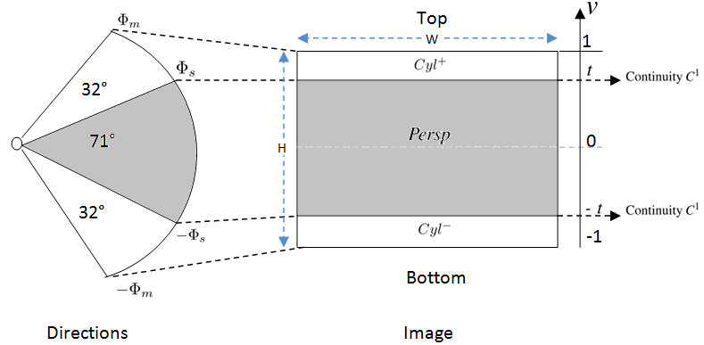
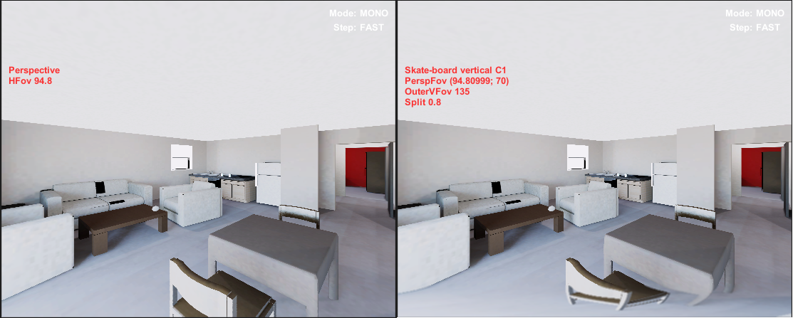
| − | + | Image:boustila_2016_a_hybrid_projection_to_widen_the_vertical_field_of_view_with_large_screens.png | '''A Hybrid Projection to Widen the Vertical Field of View with Large Screens :''' Left image represents a view with a perspective projection. Right image shows and example of the hybrid projection. In left image the user cannot see the chair behind him. [https://icube-publis.unistra.fr/docs/9976/3DUI2016.pdf [3DUI-2016]] | |
| − | + | Image:SpidarWB.jpg | '''Materiel de réalité de synthèse :''' Spidar et workbench. | |
| − | < | + | Image:Materiel_workbench.jpg | '''Materiel de réalité de synthèse :''' Gants et wand. |
| + | Image:IncaHardware.jpg | '''Materiel de réalité de synthèse :''' INCA | ||
| + | Image:IncaHandle.jpg | '''Materiel de réalité de synthèse :''' Effecteur du périphérique haptique | ||
| + | Image:IncaTracking.jpg | '''Materiel de réalité de synthèse :''' Caméra pour suivi de position | ||
| + | Image:Rv_terrain.png | '''Edition de Terrain :''' Edition de terrain | ||
| + | Image:CCubeTerrainEdit.jpg | '''Edition de Terrain :''' CCube Menu | ||
| + | Image:9N5A1823-small.jpg | '''Edition de Terrain :''' Edition de terrain | ||
| + | Image:9N5A1819-small.jpg | '''Edition de Terrain :''' Edition de terrain | ||
| + | Image:Geolo_pilote.jpg | '''Applications géologiques :''' | ||
| + | Image:Geolo_select.jpg | '''Applications géologiques :''' | ||
| + | Image:Geolo_wb.jpg | '''Applications géologiques :''' | ||
| + | Image:WbMultiRes2.jpg | '''Edition multi-resolution en Réalité Virtuelle :''' | ||
| + | Image:WbMultiRes3.jpg | '''Edition multi-resolution en Réalité Virtuelle :''' | ||
| + | Image:9N5A1803-small.jpg | '''Edition multi-resolution en Réalité Virtuelle :''' | ||
| + | Image:9N5A1805-small.jpg | '''Edition multi-resolution en Réalité Virtuelle :''' | ||
| + | Image:9N5A1773-small.jpg | '''Visualisation d'objet numérisé en environnement immersif :''' | ||
| + | Image:9N5A1770-small.jpg | '''Visualisation d'objet numérisé en environnement immersif :''' | ||
| + | Image:9N5A1811-small.jpg | '''Visualisation de modèle médical en environnement immersif :''' | ||
| + | Image:9N5A1812-small.jpg | '''Visualisation de modèle médical en environnement immersif :''' | ||
| + | Image:Principle.png | '''Facteurs de perception des distances en environnement virtuel :''' Le principe de la projection hybride et les différents paramètres utilisés pour le rendu de la scène. | ||
| + | Image:Projection_example_1.png | '''Facteurs de perception des distances en environnement virtuel :''' Gauche : vue de scène projetée avec la projection perspective ordinaire. Droite : un exemple de la même vue avec la projection hybride. Sur l'image de gauche l'utilisateur ne voit pas les pieds de la chaise devant lui. | ||
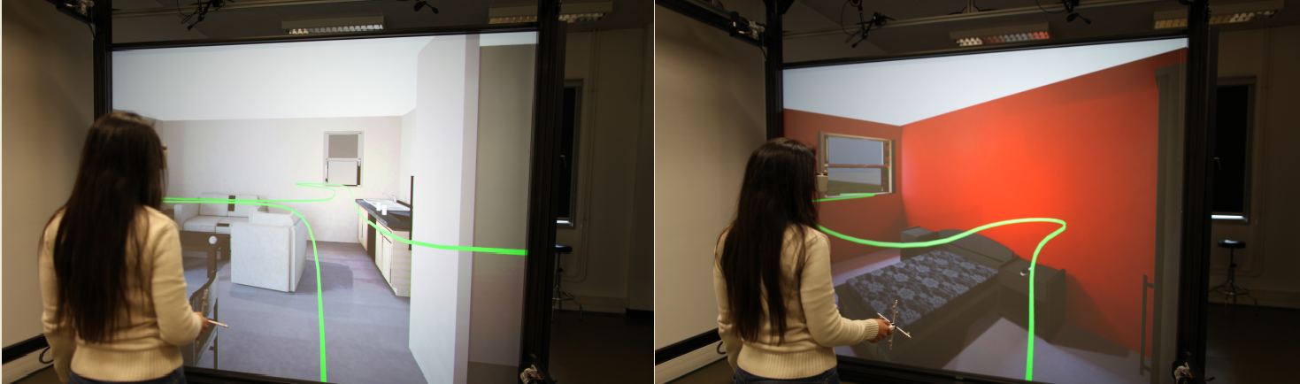
| + | Image:Virtual_visit.png | '''Facteurs de perception des distances en environnement virtuel :''' Exemple de visite virtuelle : des positions différentes lors de la visite d'une maison meublée. Le chemin de navigation est représenté en fil d'Ariane en vert. | ||
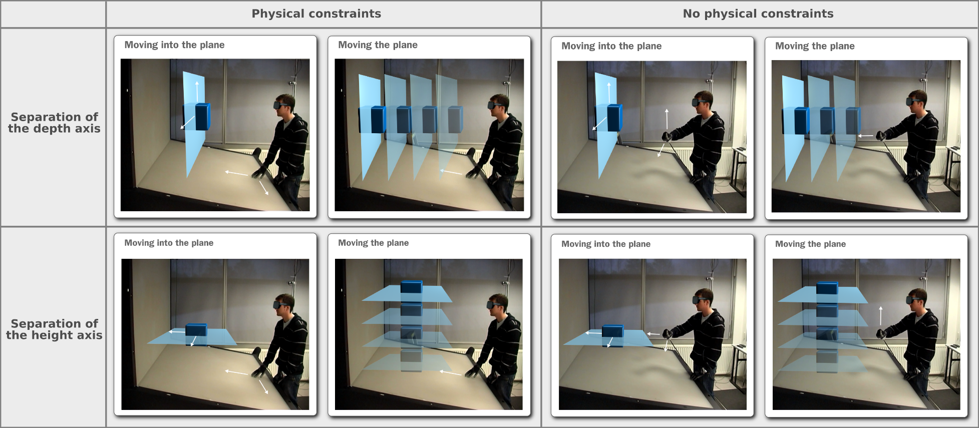
| + | Image:DLL_splitting.png | '''Séparation des degrés de liberté pour la manipulation d'objets :''' Etude de l'impact de la séparation des degrés de liberté pour l'interaction en environnement immersif. | ||
| + | </gallery> | ||
| + | == Modélisation == | ||
| − | == | + | <gallery mode="packed-hover" heights="200px"> |
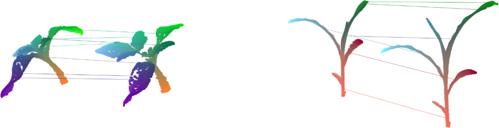
| − | + | Image:pan_2021_multi_scale_space_time_registration_of_growing_plants_00.png | '''Multi-scale Space-time Registration of Growing Plants :''' Result of our framework on one tomato plant (left) and one maize (right): corresponding points share the same colour. Some landmarks have been sampled and are shown connected to their corresponding points. [https://icube-publis.unistra.fr/docs/15504/3dv_paper.pdf [3DV-2021]] | |
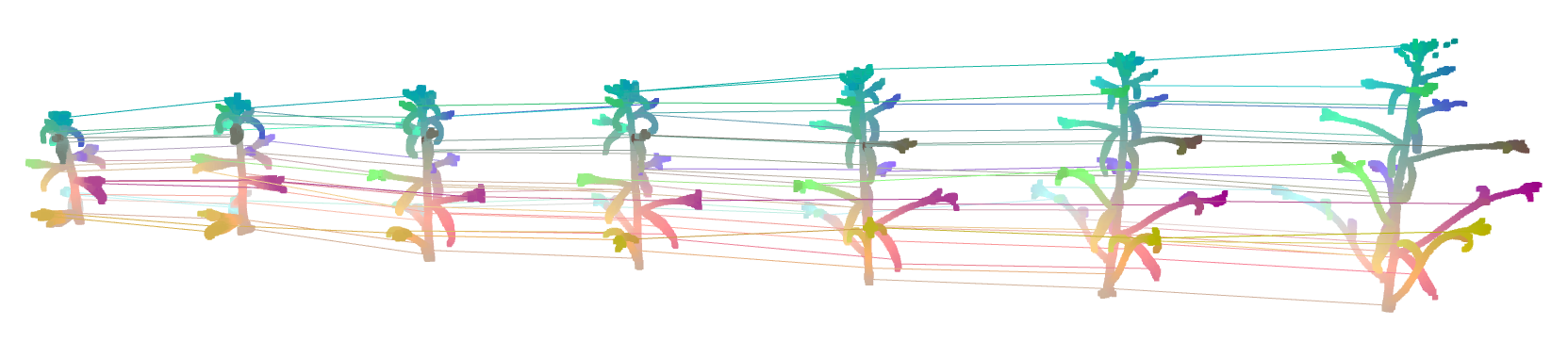
| − | + | Image:pan_2021_multi_scale_space_time_registration_of_growing_plants_01.png | '''Multi-scale Space-time Registration of Growing Plants :''' Point-wise matching of the whole plant growing. [https://icube-publis.unistra.fr/docs/15504/3dv_paper.pdf [3DV-2021]] | |
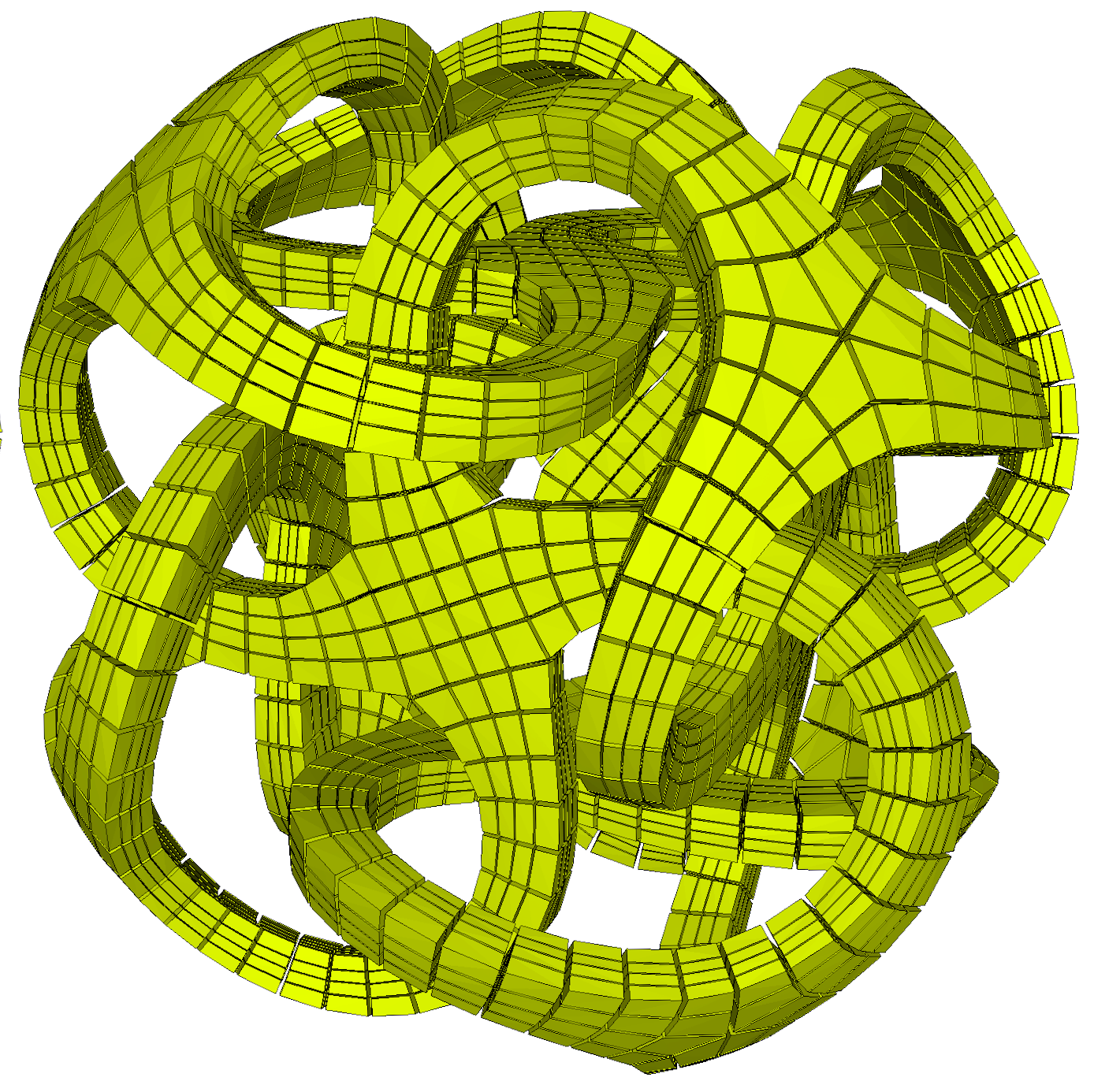
| − | + | Image:viville_2021_hexahedral_mesh_generation_for_tubular_shapes_using_skeletons_and_connection_surfaces_00.png | '''Tubular shape scaffolding :''' Hexahedral reconstruction of the metatron mesh using the tubular shape scaffolding algorithm. [https://icube-publis.unistra.fr/4-VKB21 [VISIGRAPP-2021]] | |
| − | + | Image:viville_2021_hexahedral_mesh_generation_for_tubular_shapes_using_skeletons_and_connection_surfaces_01.png | '''Tubular shape scaffolding :''' Using the red scaffold as a support a hexahedral mesh is produced then optimized and fitted to the input surface. [https://icube-publis.unistra.fr/4-VKB21 [VISIGRAPP-2021]] | |
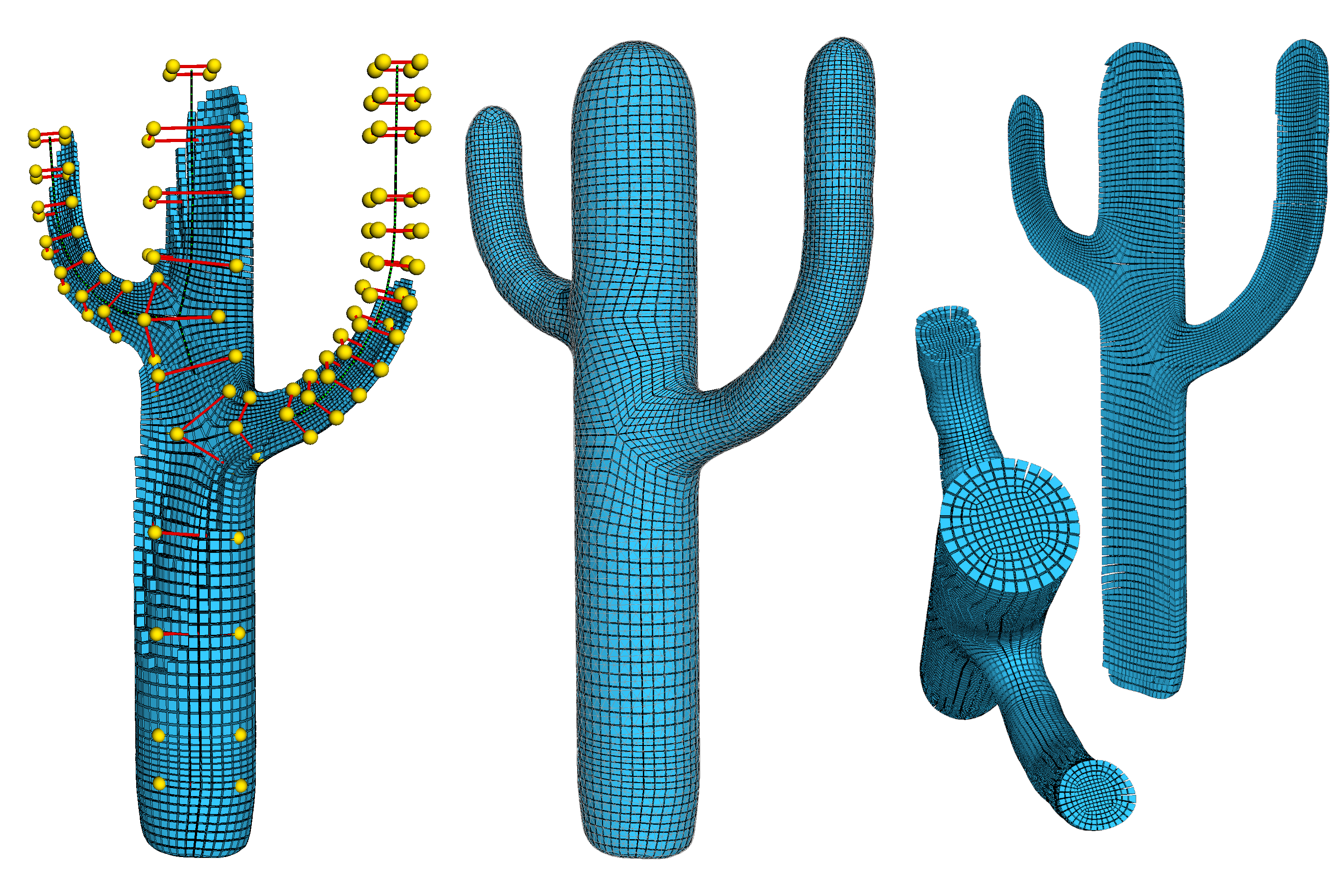
| − | < | + | Image:viville_2021_hexahedral_mesh_generation_for_tubular_shapes_using_skeletons_and_connection_surfaces_02.png | '''Hex Meshes :''' Construction of hexahedral meshes (yellow) from an input surface (blue) and it's curve skeleton using the scaffold method. [https://icube-publis.unistra.fr/4-VKB21 [VISIGRAPP-2021]] |
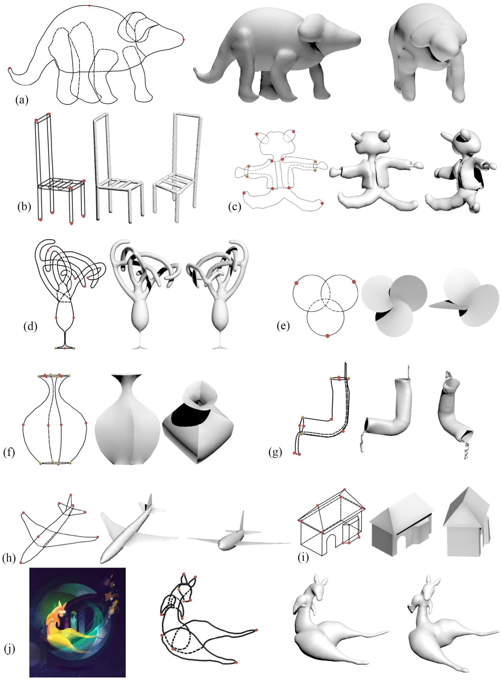
| + | Image:bobenrieth_2020_descriptive_interactive_3d_shape_modeling_from_a_single_descriptive_sketch.png | '''Descriptive: Interactive 3D Shape Modeling from A Single Descriptive Sketch :''' The constraints specified by the user are shown in red for positional constraints green for corner points and green–red for both. [https://icube-publis.unistra.fr/docs/14544/Descriptive.pdf [CAD-2020]] | ||
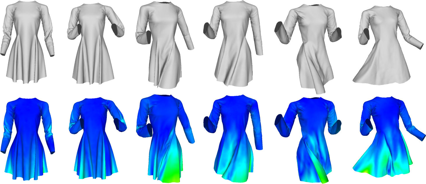
| + | Image:yang_2018_analyzing_clothing_layer_deformation_statistics_of_3d_human_motion.png | '''Analyzing Clothing Layer Deformation Statistics of 3D Human Motions :''' Comparison to ground truth. First row: our predicted clothing deformation. Second row: ground truth colored with per-vertex error. Blue: 0cm; red: 10cm. [https://icube-publis.unistra.fr/docs/13307/yang2018analyzing.pdf [ECCV-2018]] | ||
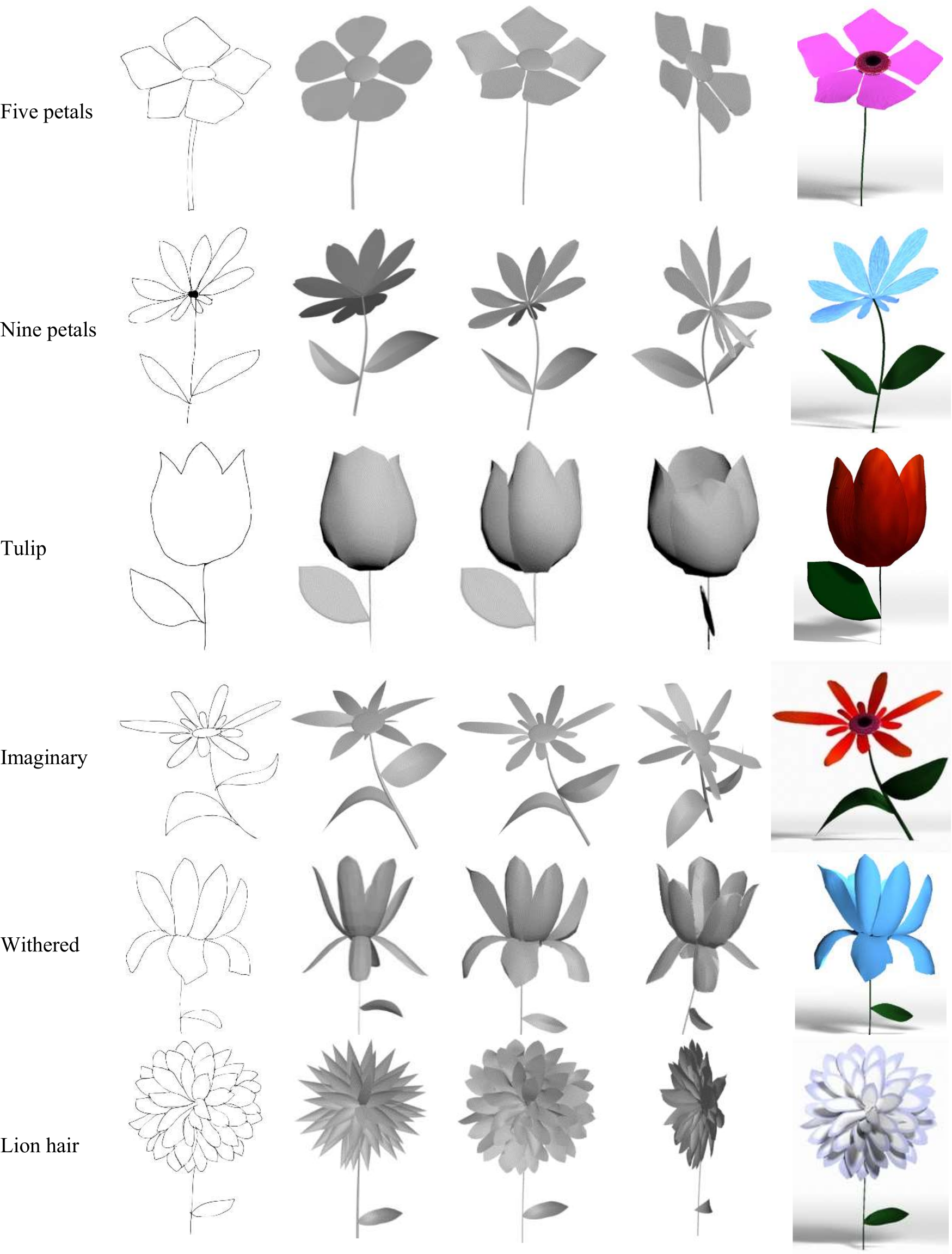
| + | Image:bobenrieth_2018_reconstructiong_flowers_from_sketches_00.png | '''Reconstructing Flowers from Sketches :''' Reconstruction of a flower model from a sketch: input sketch (a); guide strokes provided by the user (b); segmented sketch into petals and other botanical elements (c); reconstructed model (d and e). [https://icube-publis.unistra.fr/docs/13320/Reconstructing%20Flowers%20from%20Sketches.pdf [PG-2018]] | ||
| + | Image:bobenrieth_2018_reconstructiong_flowers_from_sketches_01.png | '''Reconstructing Flowers from Sketches :''' Results obtained with our modeler. [https://icube-publis.unistra.fr/docs/13320/Reconstructing%20Flowers%20from%20Sketches.pdf [PG-2018]] | ||
| + | Image:bobenrieth_2018_reconstructiong_flowers_from_sketches_02.png | '''Reconstructing Flowers from Sketches :''' More flower model examples from our modeler. [https://icube-publis.unistra.fr/docs/13320/Reconstructing%20Flowers%20from%20Sketches.pdf [PG-2018]] | ||
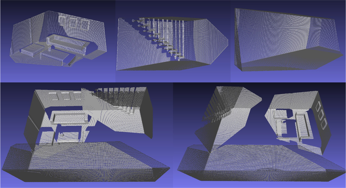
| + | Image:bobenrieth_2017_indoor_scene_reconstruction_from_a_sparse_set_of_3d_shots.png | '''Indoor Scene reconstruction from a sparse set of 3D shots :''' Three shots containing no overlapping area are given as input (top row). The second row shows two different results provided by our method. [https://icube-publis.unistra.fr/docs/12967/IndoorSceneReconstruction.pdf [CGI-2017]] | ||
| + | Image:paulus_2016_handling_topological_changes_during_elastic_registration.png | '''Handling Topological Changes during Elastic Registration :''' Augmented reality on cut and deformed kidney 1 (top) and 2 (bottom) overlaid by the virtual organ the initial registration (left) final registrations: uncut (middle left) cut (middle right) and reference registration (right). [https://hal.inria.fr/hal-01397409/document [IJCARS-2016]] | ||
| + | Image:chen_2016_mesh_sequence_morphing.png | '''Mesh Sequence Morphing :''' A galloping Camel gradually changes into a galloping Dino. The Dino sequence (indicated in blue) is obtained by transferring the deformations of the Camel to the compatibly remeshed Dino in the rest pose. [https://icube-publis.unistra.fr/docs/9060/CGF2016Vol35Number1pp179-190.pdf [CGF-2016]] | ||
| + | Image:lung_mesh.png | '''Animation de bronches :''' Construction d'un maillage volumique hexaédrique d'un modèle de bronches | ||
| + | Image:lung_anim.png | '''Animation de bronches :''' Cycle de respiration sur un maillage volumique de bronches. | ||
| + | Image:OpenStreetMapImport.png | '''Simulation de foule :''' Données géographiques importées depuis open street map. | ||
| + | Image:CrowdOnFloor.png | '''Simulation de foule :''' Bâtiments composés d'étages. | ||
| + | Image:CrowdOnPlanet.png | '''Simulation de foule :''' Foule sur une planète virtuelle. | ||
| + | Image:CrowdOnKnoth.png | '''Simulation de foule :''' Support de topologies extrêmes. | ||
| + | Image:CPH_2D.png | '''Modèle volumique adaptatif et multirésolution :''' Labellisation des cellules pour définir une hiérarchie implicite. | ||
| + | Image:Volume_subdivision.png | '''Modèle volumique adaptatif et multirésolution :''' Subdivision volumique d'un tore à trois trous modélisé par un ensemble de polyèdres quelconques. | ||
| + | Image:Pierre_cube_catmullclark.jpg | '''Modélisation multi-résolution :''' Utilisation des MR-Maps dans un outil d'édition multirésolution avec des surfaces de subdivision multirésolution générées avec le schéma de Catmull-Clark (maillage carré). | ||
| + | Image:Pierre_horse_quadtriangle.jpg | '''Modélisation multi-résolution :''' Utilisation des MR-Maps dans un outil d'édition multirésolution avec des surfaces de subdivision multirésolution générées avec le schéma Quad - Triangle (maillage hybride triangle - carré). | ||
| + | Image:Pierre_bunny_sqrt3.jpg | '''Modélisation multi-résolution :''' Utilisation des MR-Maps dans un outil d'édition multirésolution avec des surfaces de subdivision multirésolution générées avec le schéma Sqrt(3) (schéma de Kobbelt). | ||
| + | Image:Dobrina_lapins.jpg | '''Reconstruction de maillages à partir d'images voxels :''' Trois étapes clés de l'algorithme de reconsctruction Delaunay Discret a) Approximation discrète des régions de Voronoï sur la frontière discrète b) Graphe de Voronoï discret c) Reconstruction par dualité : graphe de Voronoi euclidien (en noir). | ||
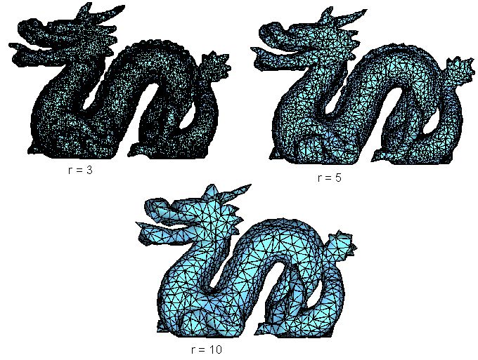
| + | Image:Dobrina_dragons.jpg | '''Reconstruction de maillages à partir d'images voxels :''' Reconstruction surfacique du fameux objet dragon avec trois résolutions différentes. | ||
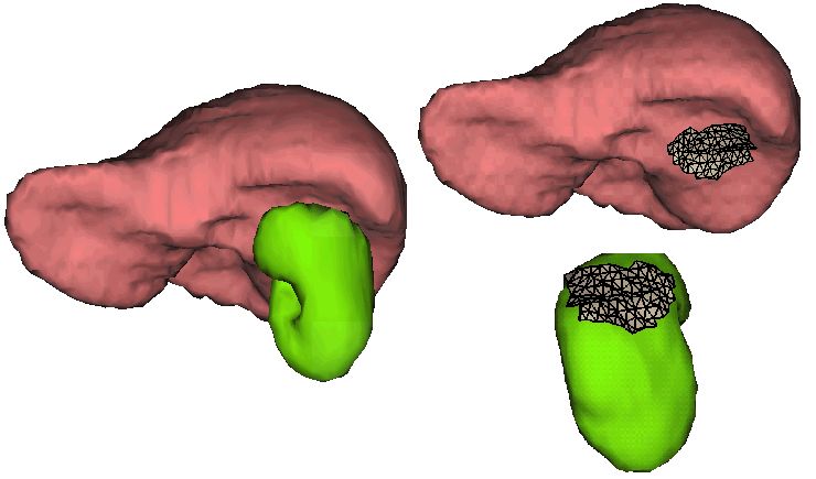
| + | Image:Dobrina_simultane.jpg | '''Reconstruction de maillages à partir d'images voxels :''' Reconstruction simultanée du foie et du rein droit. La frontière commune est contenue dans les deux maillages. | ||
| + | Image:Dobrina_bones-aorte.jpg | '''Reconstruction de maillages à partir d'images voxels :''' Exemple de reconstruction d'un squelette et d'une aorte. | ||
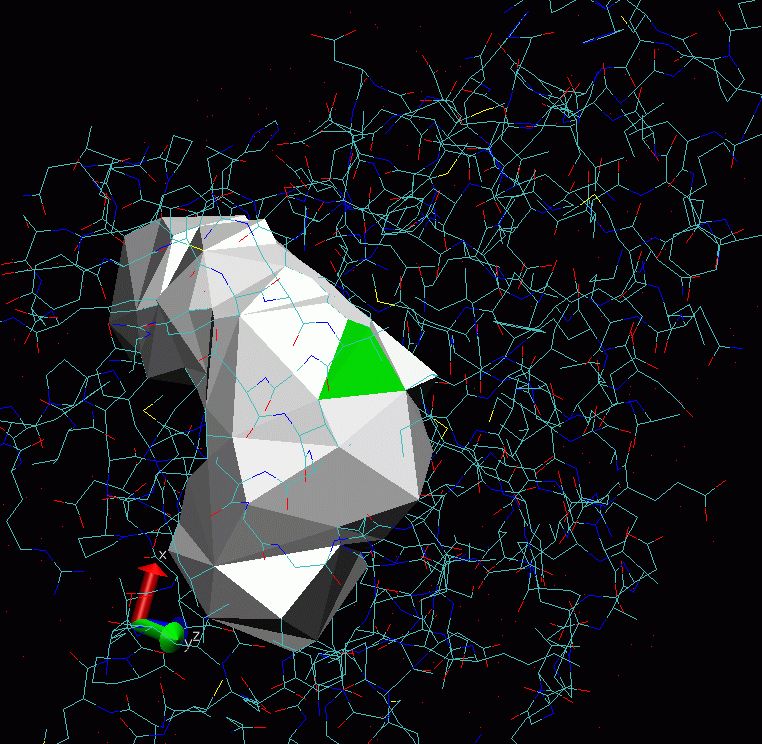
| + | Image:Schwartz1.jpg | '''Détection et caractérisation des poches dans les protéines :''' Un polygone transparent met en évidence la poche principale du domaine de liaison du ligand du récepteur à la vitamine D. on peut distinguer un ligand modélisé par une union de sphères. | ||
| + | Image:Schwartz3.jpg | '''Détection et caractérisation des poches dans les protéines :''' Même protéine et même poche sans transparence cette fois. Les facettes vertes représentent un passage bloqué entre deux poches voisines. Cette information est importante pour le biologiste. | ||
| + | Image:Vaiss_0.png | '''Modélisation de vaisseaux :''' | ||
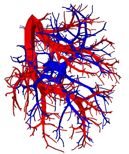
| + | Image:Vaiss_1.jpg | '''Modélisation de vaisseaux :''' Réseau vasculaire du foie reconstruit (topologiquement). | ||
| + | Image:Vaiss_2.jpg | '''Modélisation de vaisseaux :''' Réseau vasculaire reconstruit (topologiquement). | ||
| + | Image:FilArianne.jpg | '''Navigation dans les vaisseaux :''' Chemin dans un vaisseau. | ||
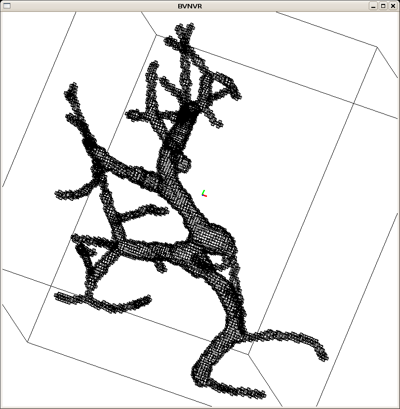
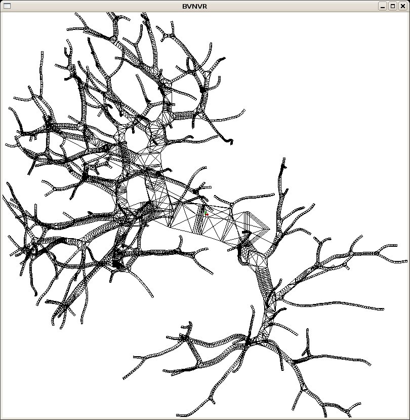
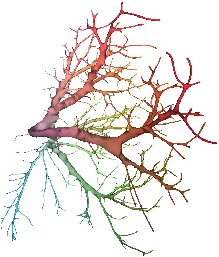
| + | Image:BV-Rainbow.jpg | '''Navigation dans les vaisseaux :''' Réseau de vaisseau. | ||
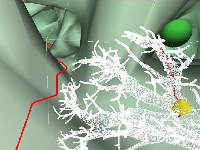
| + | Image:Capture-NavigWIM.jpg | '''Navigation dans les vaisseaux :''' Aide à la navigation. | ||
| + | Image:Visu-In-Uni.jpg | '''Navigation dans les vaisseaux :''' Visualisation de l'intérieur des vaisseaux. | ||
| + | Image:Multifil_fleur.jpg | '''Modélisation topologie et plongement (Multifil) :''' | ||
| + | Image:Multifil_lotus7.jpg | '''Modélisation topologie et plongement (Multifil) :''' | ||
| + | Image:Multifil_telephone.jpg | '''Modélisation topologie et plongement (Multifil) :''' | ||
| + | Image:Multifil_cuisine.jpg | '''Modélisation topologie et plongement (Multifil) :''' | ||
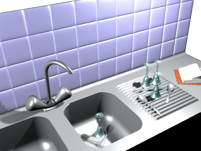
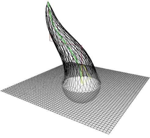
| + | Image:Dogme corne.jpg | '''Modèles de déformation :''' Dogme. | ||
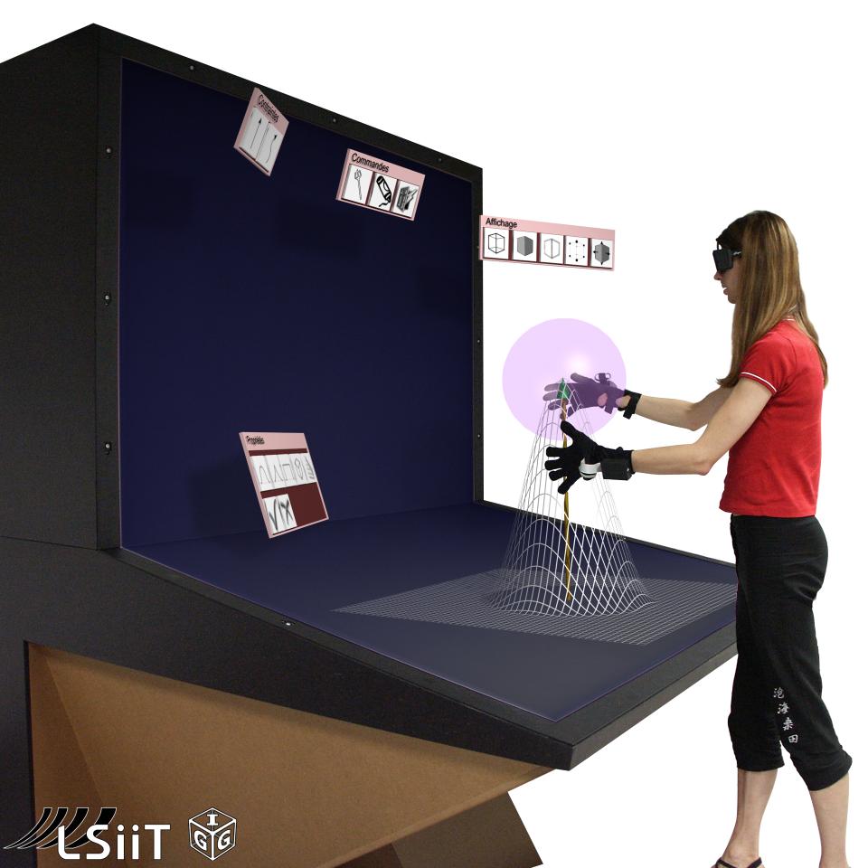
| + | Image:Dogmerv.jpg | '''Modèles de déformation :''' Dogme en réalité virtuelle. | ||
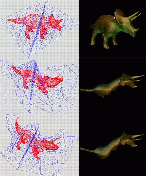
| + | Image:Dinosaure.png | '''Modèles de déformation :''' CFFD. | ||
| + | Image:ISMAR2015_teaser.png | '''Simulation de découpes et déchirures en temps réel :''' Vue augmentée d'un objet élastique supportant de fortes déformations et des changements topologiques. | ||
| + | Image:Liver-AR-01.png | '''Simulation de découpes et déchirures en temps réel :''' Vue augmentée d'une séquence opératoire en milieu médical. | ||
| + | Image:ARinOR.png | '''Simulation de découpes et déchirures en temps réel :''' Vue augmentée d'une séquence opératoire en milieu médical. | ||
| + | Image:Img_featurepoints.png | '''Analyse des formes - recalage - segmentation de données dynamiques :''' Extraction de points caractéristiques à l'aide de notre technique AniM-DoG sur différentes poses de maillages animés. La couleur représente l'échelle temporelle des points caractéristiques; le rayon indique l'échelle spatiale. | ||
| + | Image:Img_spatialmatching.png | '''Analyse des formes - recalage - segmentation de données dynamiques :''' Pour un couple de maillages animés avec des mouvements similaires sémantiquement nous calculons un ensemble de points caractéristiques sur chaque maillage et leur correspondances spatiales. | ||
| + | </gallery> | ||
| − | = | + | == Spécification et preuves == |
| − | == | + | <gallery mode="packed-hover" heights="200px"> |
| − | + | Image:desargues2d.png | '''Spécifications et preuves :''' | |
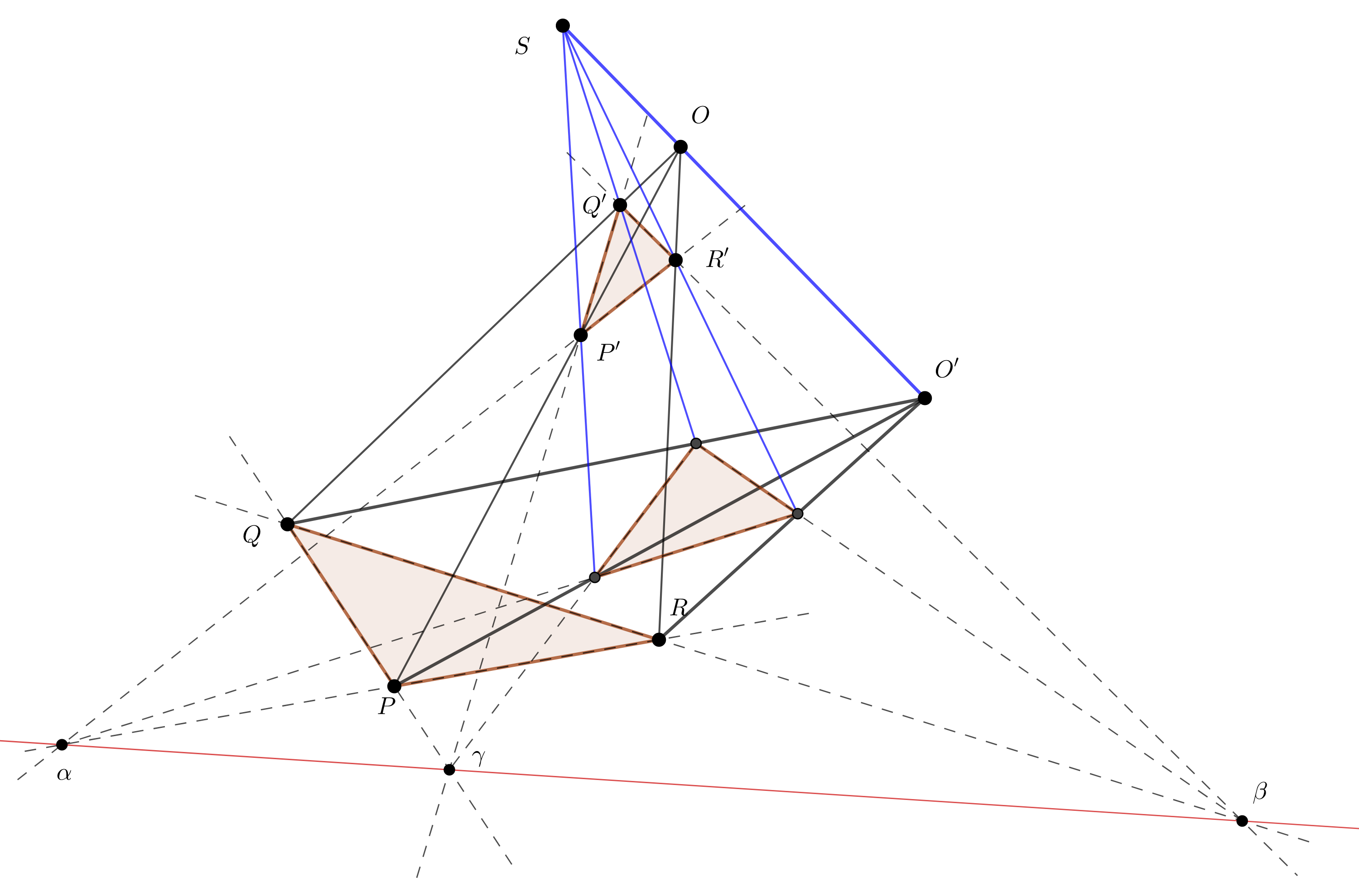
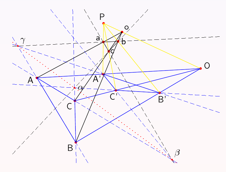
| − | + | Image:desargues_3D_plan.png | '''Spécifications et preuves :''' Illustration 3D du théorème de Desargues dans un espace projectif de dimension 3 : les cotés correspondants de 2 tétraèdres en perspective l'un de l'autre se coupent en 6 points coplanaires (ces six points forment un quadrilatère complet). | |
| − | + | Image:Jfd_hmap1.png | '''Spécifications et preuves :''' | |
| − | + | Image:Jfd_hmap1Torus.png | '''Spécifications et preuves :''' | |
| − | < | + | Image:Jfd_hmap2.png | '''Spécifications et preuves :''' |
| + | Image:Jfd_polyhedra1.png | '''Spécifications et preuves :''' | ||
| + | Image:Jfd_nf.png | '''Spécifications et preuves :''' | ||
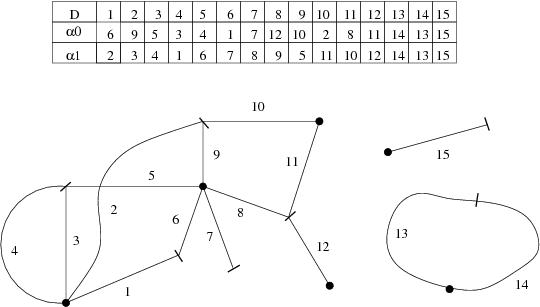
| + | Image:Jfd_seg_subd1seg.png | '''Certification d'une segmentation d'image modélisée par hypercartes colorées :''' Une subdivision du plan colorée (avec un sommet isolé et des arêtes pendantes) et sa segmentation. | ||
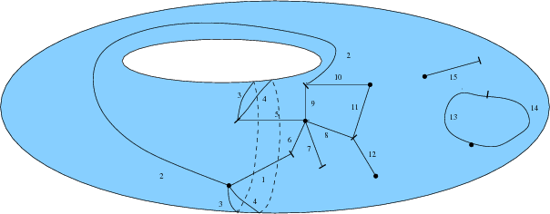
| + | Image:Jfd_seg_hmap2.png | '''Certification d'une segmentation d'image modélisée par hypercartes colorées :''' Modélisation de la subdivision précédente par une quasi-hypercarte (sommets ou arêtes ouverts). | ||
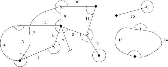
| + | Image:Jfd_seg_hmap3.png | '''Certification d'une segmentation d'image modélisée par hypercartes colorées :''' Modélisation de la subdivision précédente par une hypercarte (sommets et arêtes fermés). | ||
| + | Image:Jfd_seg_hmap2seg.png | '''Certification d'une segmentation d'image modélisée par hypercartes colorées :''' Segmentation de la quasi-hypercarte en 2 phases (des défauts subsistent). | ||
| + | Image:Jfd_seg_hmap3seg.png | '''Certification d'une segmentation d'image modélisée par hypercartes colorées :''' Segmentation de l'hypercarte en 2 phases (le résultat est correct). | ||
| + | Image:Desargues.png | '''Illustration du théorème de Desargues :''' | ||
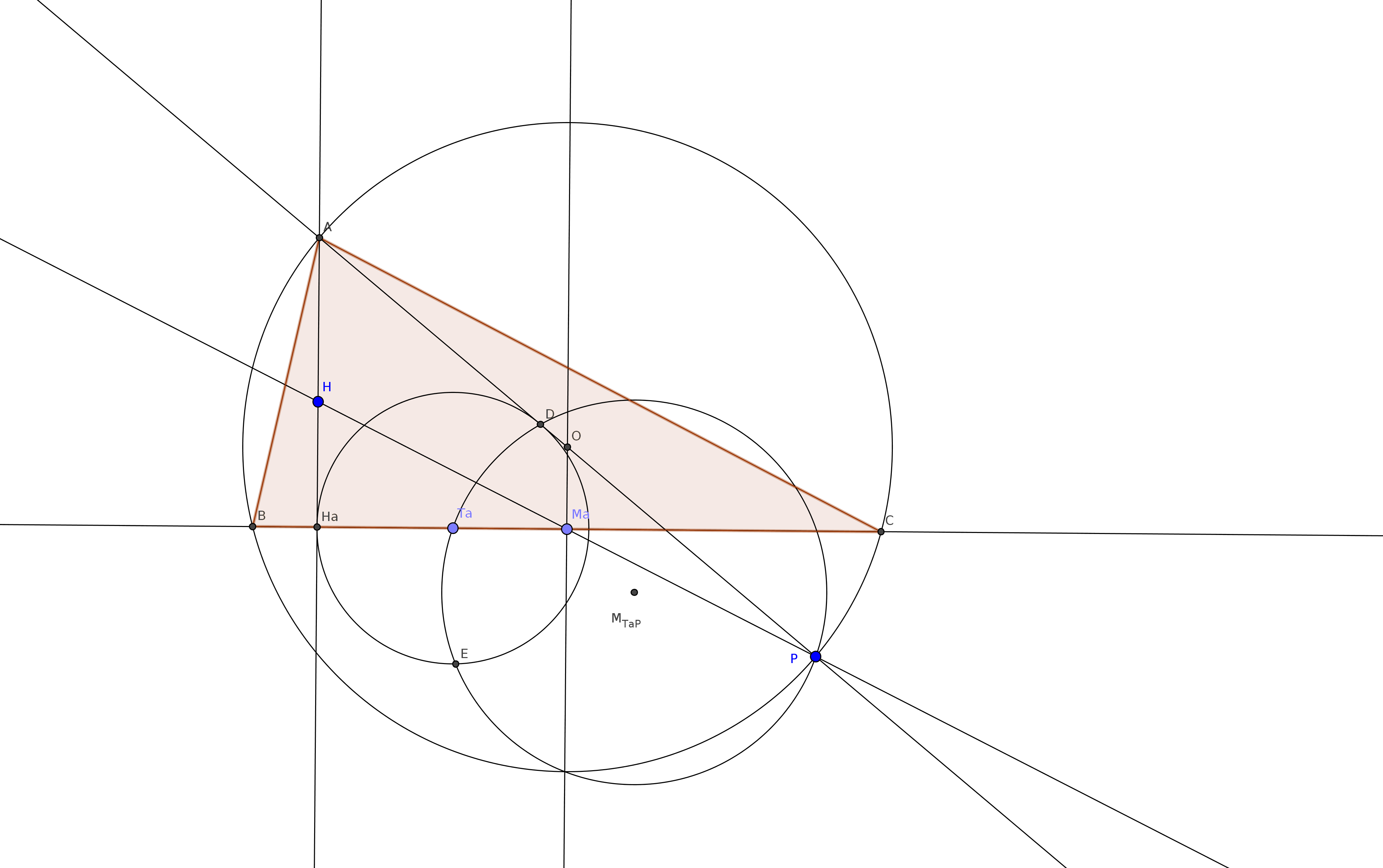
| + | Image:Wernick108RC.png | '''Construction de solutions :''' Traduction géométrique d’une solution trouvée algébriquement. | ||
| + | Image:W108Geo.png | '''Construction de solutions :''' Construction directe. | ||
| + | </gallery> | ||
| − | ==Visualisation | + | == Visualisation == |
| − | |||
| − | |||
| − | |||
| − | |||
| − | == | + | <gallery mode="packed-hover" heights="200px"> |
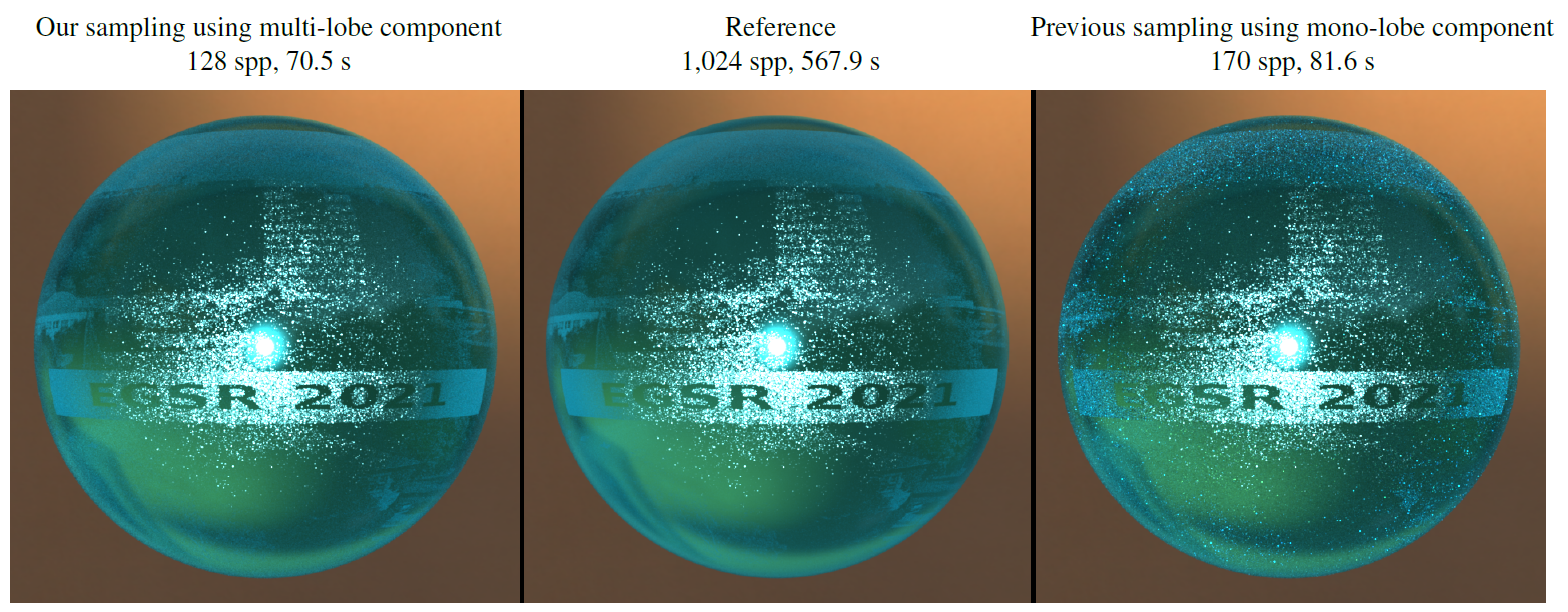
| − | + | Image:Chermain2021ImportanceSampling.png | '''Importance Sampling of Glittering BSDFs based on Finite Mixture Distributions :''' A glittering coloured glass sphere with a spatially varying microfacet density. Left: our sampling scheme. Centre: reference. Right: Gaussian mono-lobe approximation is used for sampling. [http://igg.unistra.fr/People/chermain/importance_sampling_glint/ [EGSR-2021]] | |
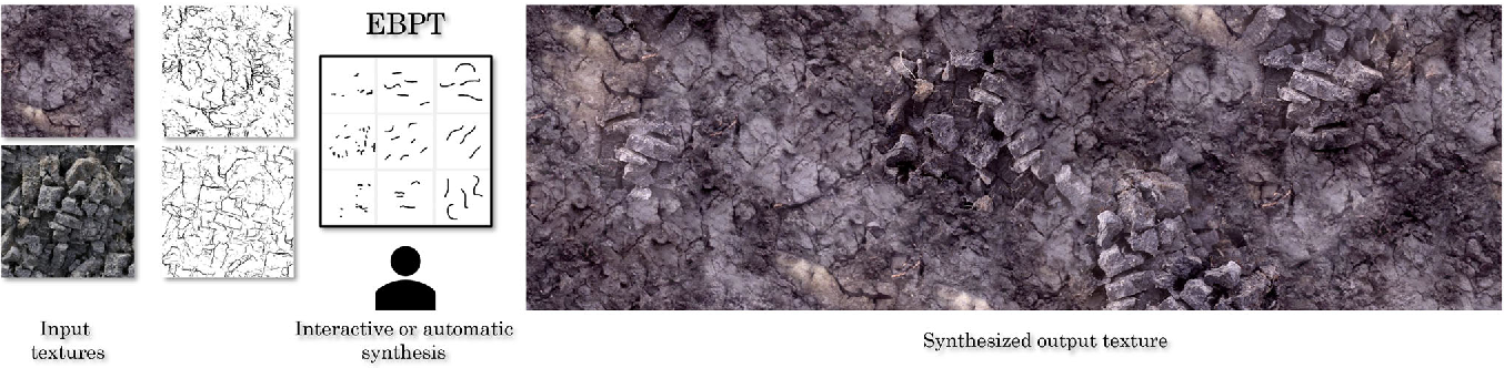
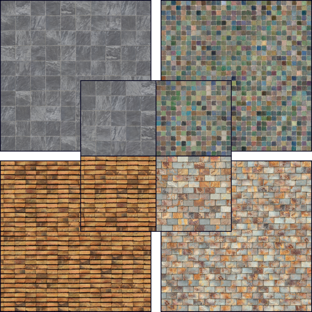
| − | + | Image:kim_2021_edge_based_procedural_textures.png | '''Edge-based procedural textures :''' Edges of a texture are extracted and encoded into an edge-based procedural texture (EBPT). New textures are generated either automatically or by controlling the EBPT generation by the user. [https://www.semanticscholar.org/paper/Edge-based-procedural-textures-Kim-Dischler/55aebfb8e9b1851de1f5e586fd64c5c869b346c8 [VC-2021]] | |
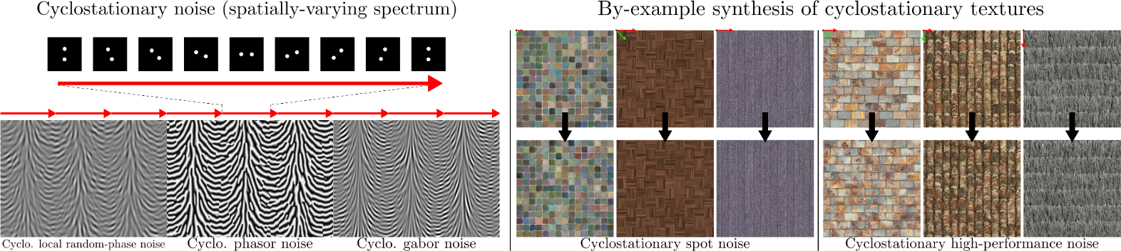
| − | + | Image:lutz_2021_cyclostationary_gaussian_noise_theory_and_synthesis.png | '''Cyclostationary Gaussian noise: theory and synthesis :''' We convey existing stationary noises to a cyclostationary context enabling the synthesis of cyclostationary textures controlled by spectra (left) and by an exemplar (right). [https://hal.archives-ouvertes.fr/hal-03181139/document [EG-2021]] | |
| − | + | Image:Chermain2020ProceduralTeaser.png | '''Procedural Physically based BRDF for Real-Time Rendering of Glints :''' Left: sparkling fabrics are rendered (3.0 ms/frame). Right: plane with specular microfacet density increasing. Top: our physically based BRDF (2.5 ms/frame). Bottom: not physically based [ZK16] (1.3 ms/frame). [http://igg.unistra.fr/People/chermain/real_time_glint/ [PG-2020]] | |
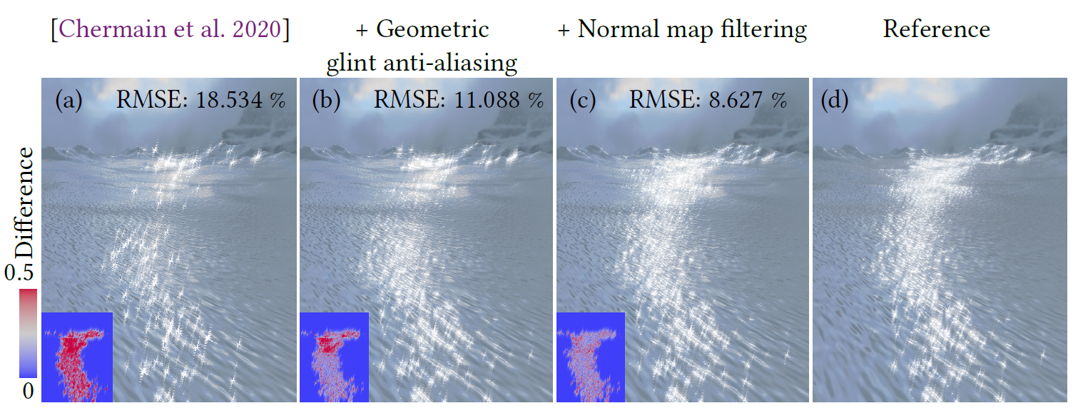
| − | + | Image:chermain2020GeometricGlint.png | '''Real-Time Geometric Glint Anti-Aliasing with Normal Map Filtering :''' Arctic landscape with a normal mapped surface. (a) glinty BRDF of Chermain et al. [2020] prone to geometric glint aliasing. Our geometric glint anti-aliasing (GGAA) without and with normal map filtering (b and c). (d) Reference. [http://igg.unistra.fr/People/chermain/glint_anti_aliasing/ [i3D-2020]] | |
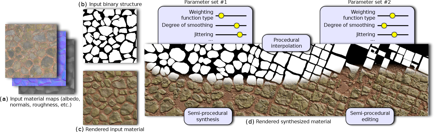
| − | + | Image:guehl_2020_semi_procedural_textures_using_point_process_texture_basis_functions.png | '''Semi-Procedural Textures Using Point Process Texture Basis Functions :''' (a) Input texture map(s) and a binary structure (b) are used to generate a semi-procedural output (d). A rendered view of the input material is shown for comparison (c). [https://icube-publis.unistra.fr/docs/14547/semiproctex_low.pdf [EGSR-2020]] | |
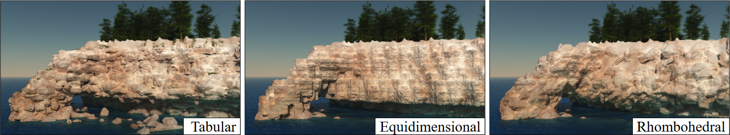
| − | + | Image:paris_2020_modeling_rocky_scenery_using_implicit_blocks.png | '''Modeling Rocky Scenery using Implicit Blocks :''' Different styles of blocks generated on a cliff and arches. From left to right tabular block style equidimensional blocks and finally rhombohedral block style. [https://hal.archives-ouvertes.fr/hal-02926218/document [VC-2020]] | |
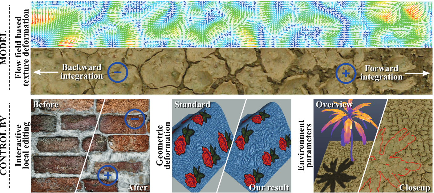
| − | + | Image:guingo_2020_content_aware_texture_deformation_with_dynamic_control.png | '''Content-aware texture deformation with dynamic control :''' Our deformation model allows to mimic non-uniform physical behaviors at texel resolution. Top: the parameterization is advected in a static flow field. Bottom: the deformation can be controlled dynamically. [https://icube-publis.unistra.fr/docs/14601/GLSLDC20.pdf [C&G-2020]] | |
| − | + | Image:lutz_2019_anisotropic_filtering_for_on_the_fly_patch_based_texturing.png | '''Anisotropic Filtering for On-the-fly Patch-based Texturing :''' Our filtering method (right) is compared to the ground truth (middle) and no filtering (left). The ground truth is computed by an exact filtering of the high resolution. The leftmost view indicates the MIP-map levels used. [https://seafile.unistra.fr/f/3ae0674a231c42818286/?dl=1 [EG-2019]] | |
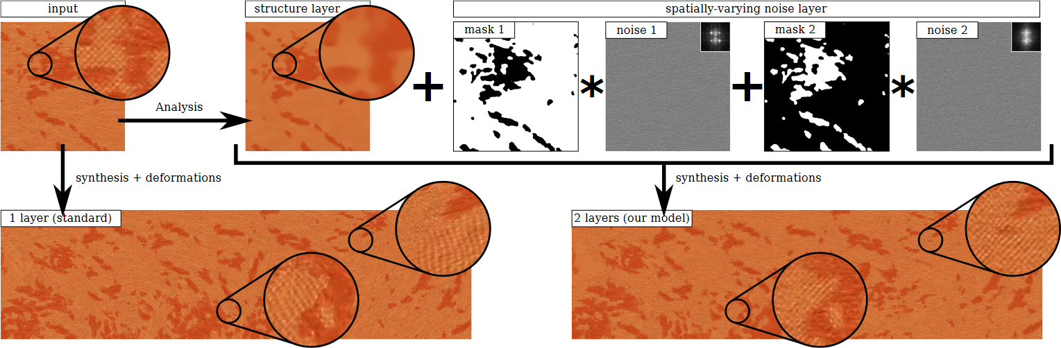
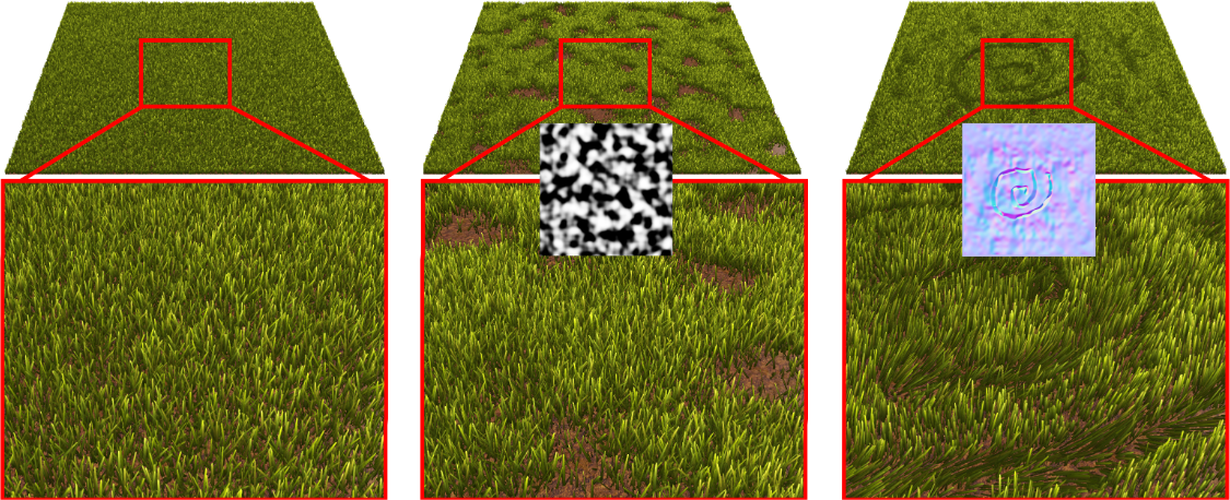
| − | + | Image:guingo_2017_bi_layer_textures.png | '''Bi-Layer textures :''' Our noise model decomposes an input exemplar as a structure layer and a noise layer. Large outputs are synthesized on-the-fly by synchronized synthesis of the layers. Variety can be achieved at the synthesis stage by deforming the structure layer while preserving fine scale appearance encoded in the noise layer. [https://hal.archives-ouvertes.fr/hal-01528537/document [EGSR-2017]] | |
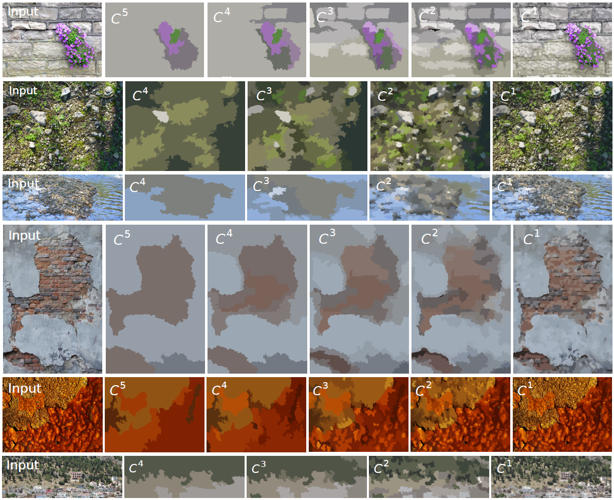
| − | + | Image:lockerman_2016_multi_scale_label_map_extraction_for_texture_synthesis.png | '''Multi-Scale Label-Map Extraction for Texture Synthesis :''' The input non-stationary texture (a). Hierarchy of labeled clusters: coarse scale (b) includes finer scales (c). Interactive texture editing (d) and content selection for creating new non-stationary textures (e). [https://graphics.cs.yale.edu/sites/default/files/multi-scale_label-map_extraction_for_texture_synthesis_low_rez.pdf [SIGGRAPH-2016]] | |
| − | + | Image:LSADDR16_Labeling_results.png | '''Modélisation et synthèse de textures :''' Des cartes de labels multi-échelles sont obtenues à l'aide de notre méthode d'analyse de textures. Une application possible est l'édition interactive de textures. [https://graphics.cs.yale.edu/sites/default/files/multi-scale_label-map_extraction_for_texture_synthesis_low_rez.pdf [SIGGRAPH-2016]] | |
| − | + | Image:pavie_2016_volumetric_spot_noise_for_procedural_3d_shell_texture_synthesis_01.png | '''Volumetric Spot Noise for Procedural 3D Shell Texture Synthesis :''' Left: uniform density. Middle: user controls density. Right: user controls orientation. In all cases control maps can be painted interactively. [https://hal.archives-ouvertes.fr/hal-02413269/document [CGVC-2016]] | |
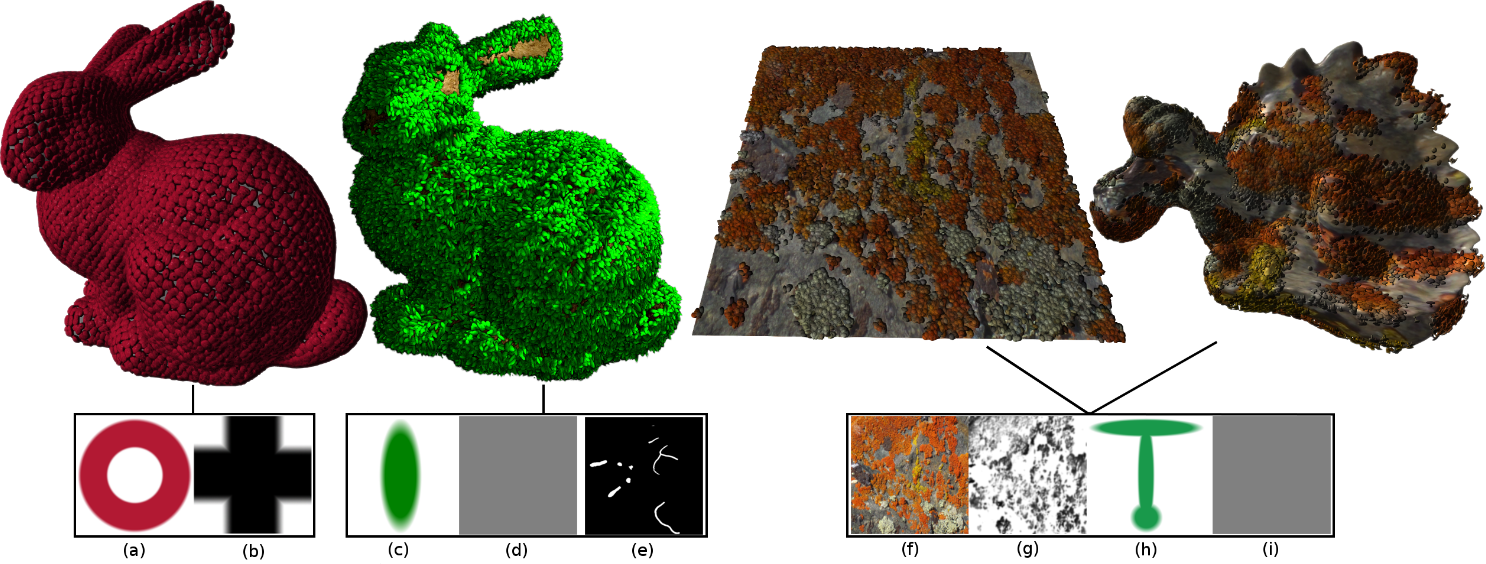
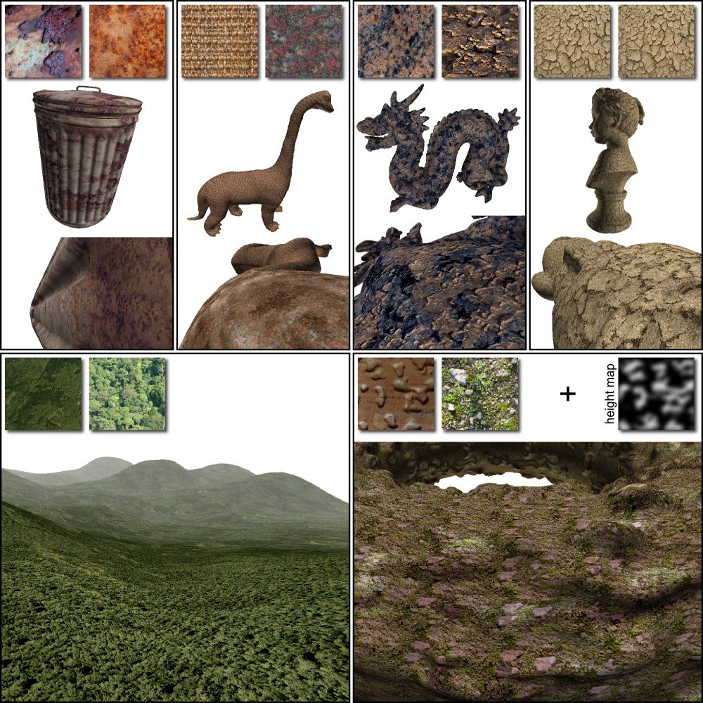
| − | + | Image:pavie_2016_volumetric_spot_noise_for_procedural_3d_shell_texture_synthesis_02.png | '''Volumetric Spot Noise for Procedural 3D Shell Texture Synthesis :''' Bunny1 with the "ring" kernel profile (a) and a semi regular distribution profile (b). Bunny2 with a Gaussian kernel profile (c) a random distribution profile (d) and a density map (e). Dragon and plan: use a color map (f) a density map (g) a kernel (h) and a random distribution (i). [https://hal.archives-ouvertes.fr/hal-02413269/document [CGVC-2016]] | |
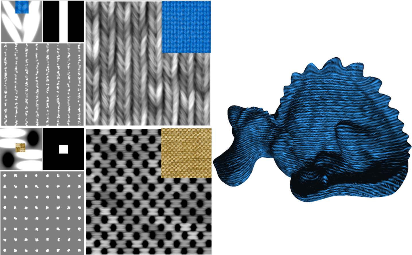
| − | + | Image:pavie_2016_procedural_texture_synthesis_by_locally_controlled_spot_noise.png | '''Procedural Texture Synthesis by Locally Controlled Spot Noise :''' Examples of a near-regular features reproduction by a single spot noise. Left: kernel profiles and distribution profiles. Right: blue fabric pattern applied on a 3D model. [file:///C:/Users/joris_r/AppData/Local/Temp/Pavie.pdf [WSCG-2016]] | |
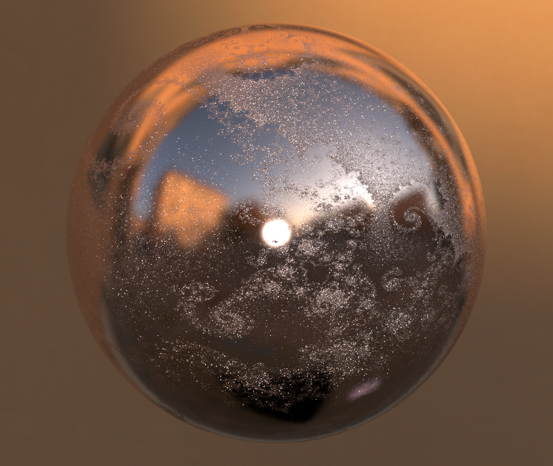
| − | + | Image:glint_cover_competition.png | '''Rendu de scintillement :''' A glittering copper sphere with spatially varying glitter density illuminated by an environment map and a point light. See [EGSR-2021]. | |
| − | + | Image:schrek2021.png | '''Synthèse cyclostationnaire de textures :''' | |
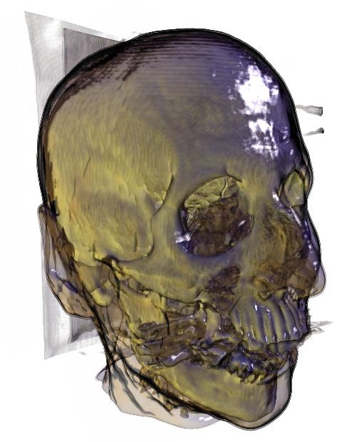
| − | + | Image:Head_our.png | '''Visualisation volumique avec éclairage :''' | |
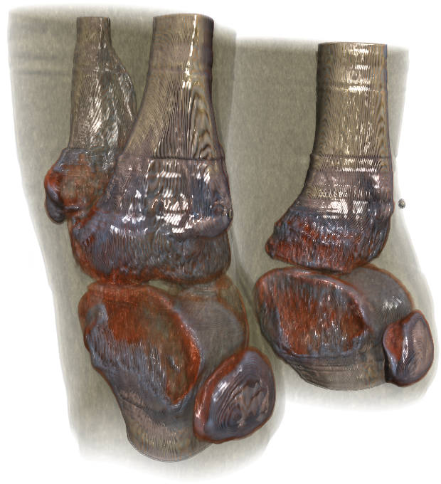
| − | + | Image:Ctknee_our.png | '''Visualisation volumique avec éclairage :''' | |
| − | + | Image:Ambientocclusion.png | '''Visualisation volumique avec éclairage :''' Occlusion ambiante. | |
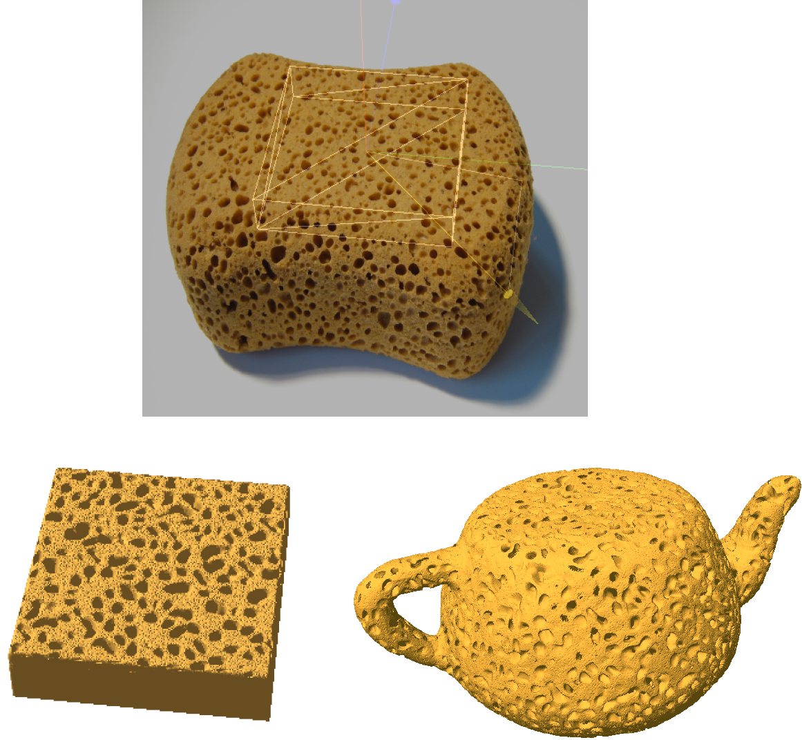
| − | + | Image:Sponge_teapot.png | '''Textures :''' Texture volumique. | |
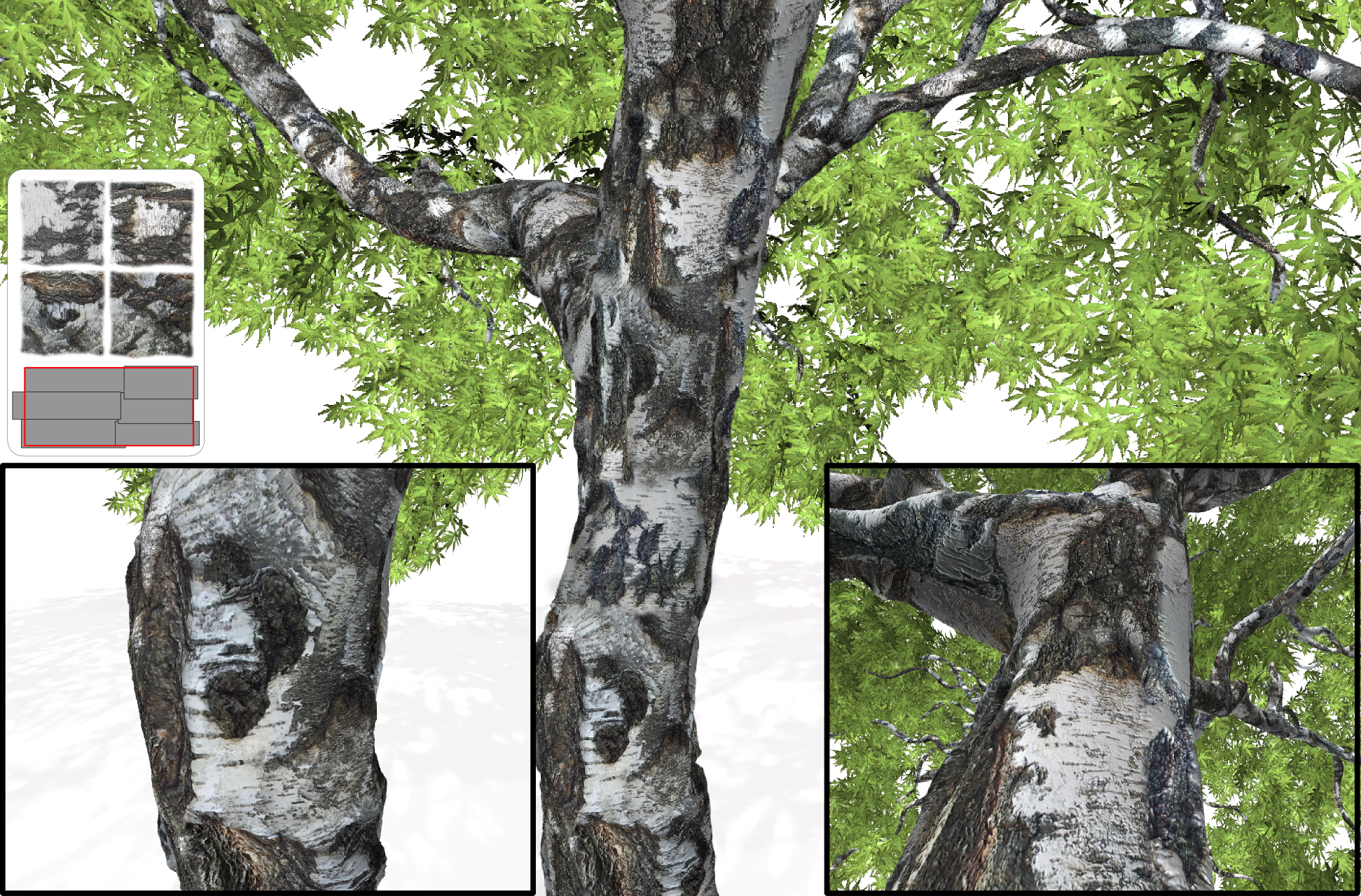
| − | + | Image:TreeF4.png | '''Textures :''' MegaTexel texture. | |
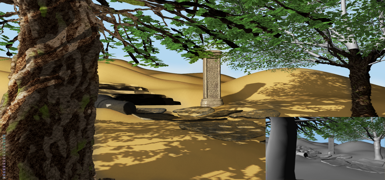
| − | + | Image:SceneFinaleRendu.png | '''Textures :''' Scène complète. | |
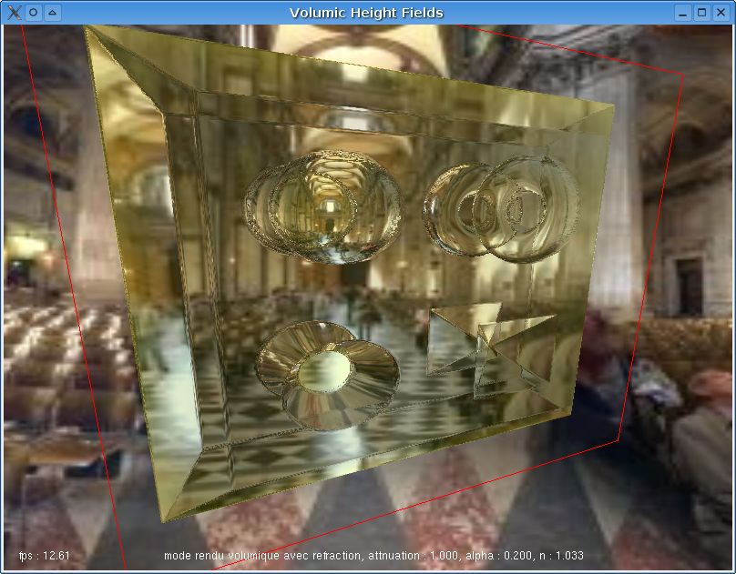
| − | + | Image:Lucas_volumiqueRefraction1.jpg | '''Visualisation volumique accélérée par GPU :''' Rendu d'objet transparent via un algorithme dérivé du relief mapping assimilable à un lancé de rayons sur un champs de hauteurs. L'objet est simplement représenté par une combinaison de cartes de hauteurs. | |
| − | + | Image:Lucas_scanHF_1.jpg | '''Visualisation volumique accélérée par GPU :''' Rendu d'un objet scanné via un algorithme de relief mapping. On s'attache ici à visualiser l'objet en exploitant directement les données issues de scanner 3D sans utiliser de. Haut : rendu obtenu. Bas : carte de hauteurs et de normales. | |
| − | + | Image:Lucas_scanHFmultipleBox_1.jpg | '''Visualisation volumique accélérée par GPU :''' Rendu via un algorithme de relief mapping d'un objet complet scanné : aucun maillage complexe n'est utilisé. Seul un cube sert de support au rendu. | |
| − | + | Image:Rendu_foie_texture.jpg | '''Visualisation :''' Rendu d'un foie texturé. | |
| − | + | Image:Rendu_textures_vb.jpg | '''Visualisation :''' | |
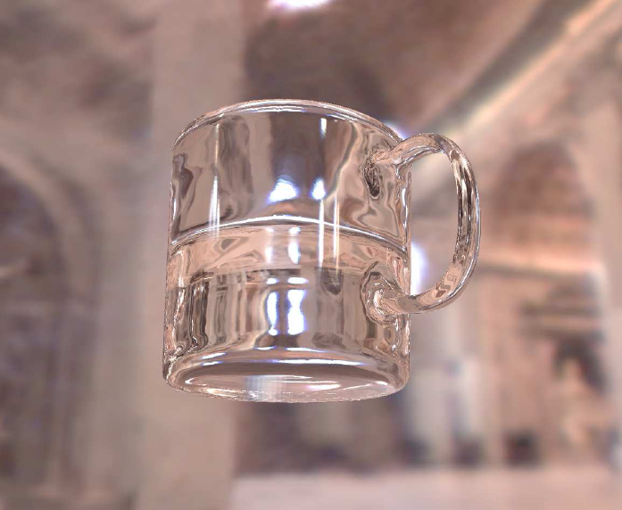
| − | + | Image:Glass.png | '''Visualisation :''' Rendu de matériau transparent. | |
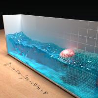
| − | + | Image:Rendu_fluide.jpg | '''Visualisation :''' Rendu de fluides. | |
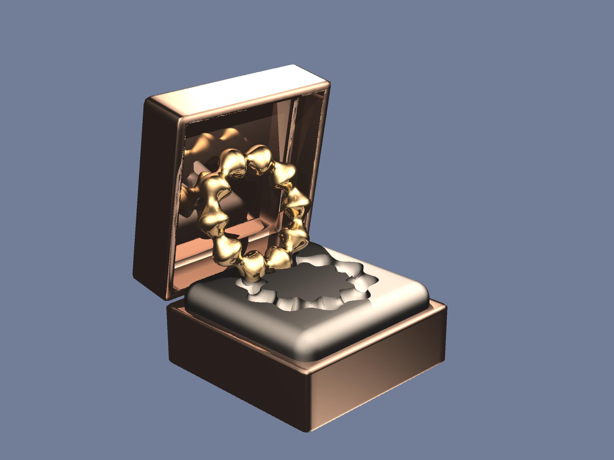
| − | + | Image:Rendu_bijou.jpg | '''Visualisation :''' Rendu de bijoux. | |
| − | + | Image:VSLD13teaser.png | '''Modélisation et synthèse de textures :''' Des textures sont synthétisées à la volée sur GPU à partir d'échantillons d'exemples à plusieurs échelles. | |
| − | + | Image:GSVDG14teaser.png | '''Modélisation et synthèse de textures :''' Des textures sont synthétisées à la volée sur GPU grâce à une analyse spectrale. | |
| − | + | </gallery> | |
| − | |||
| − | |||
| − | |||
| − | |||
| − | |||
| − | |||
| − | |||
| − | |||
| − | |||
| − | |||
| − | |||
| − | |||
| − | |||
| − | |||
| − | |||
| − | |||
| − | |||
| − | |||
| − | |||
| − | |||
| − | |||
| − | |||
| − | |||
| − | |||
| − | |||
| − | |||
| − | |||
| − | |||
| − | |||
| − | |||
| − | |||
| − | |||
| − | |||
| − | |||
| − | |||
| − | |||
| − | |||
| − | |||
| − | |||
| − | |||
| − | |||
| − | |||
| − | |||
| − | |||
| − | |||
| − | |||
| − | |||
| − | |||
| − | |||
| − | |||
| − | |||
| − | |||
| − | |||
| − | |||
| − | |||
| − | |||
| − | |||
| − | |||
| − | |||
| − | |||
| − | |||
| − | |||
| − | |||
| − | |||
| − | |||
| − | |||
| − | |||
| − | |||
| − | |||
| − | |||
| − | |||
| − | |||
| − | |||
| − | |||
| − | |||
| − | |||
| − | |||
| − | |||
| − | |||
| − | |||
| − | |||
| − | |||
| − | |||
| − | |||
| − | |||
| − | |||
| − | |||
| − | |||
| − | |||
| − | |||
| − | |||
| − | |||
| − | |||
| − | |||
| − | |||
| − | |||
| − | |||
| − | |||
| − | |||
| − | |||
| − | |||
| − | |||
| − | |||
| − | |||
| − | |||
| − | |||
| − | |||
| − | |||
| − | |||
| − | |||
| − | |||
| − | |||
| − | |||
| − | |||
| − | |||
| − | |||
| − | |||
| − | |||
| − | |||
| − | |||
| − | |||
| − | |||
| − | |||
| − | |||
| − | < | ||
| − | |||
| − | |||
Version du 15 septembre 2022 à 14:23
Acquisition

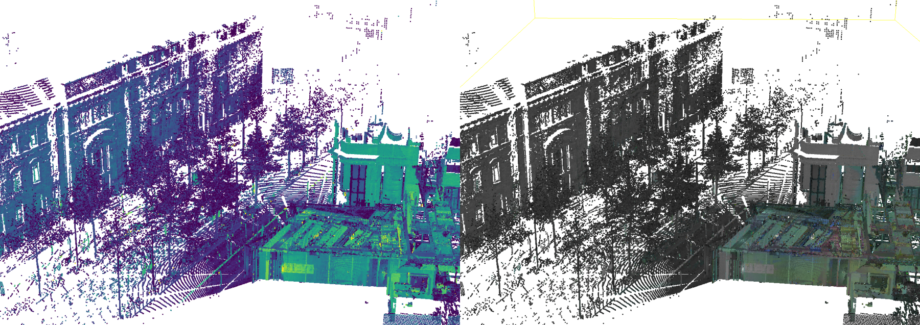
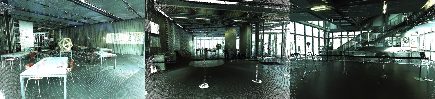
Acquisition de bâtiment à moyenne échelle : Le nuage de points de la numérisation d'une partie de l'ENSAS est coloré par intensité et par une corretion de couleur photographique.

Acquisition de bâtiment à moyenne échelle : Le nuage de points de la numérisation d'une partie de l'ENSAS est visualisé depuis trois points de vue différents.

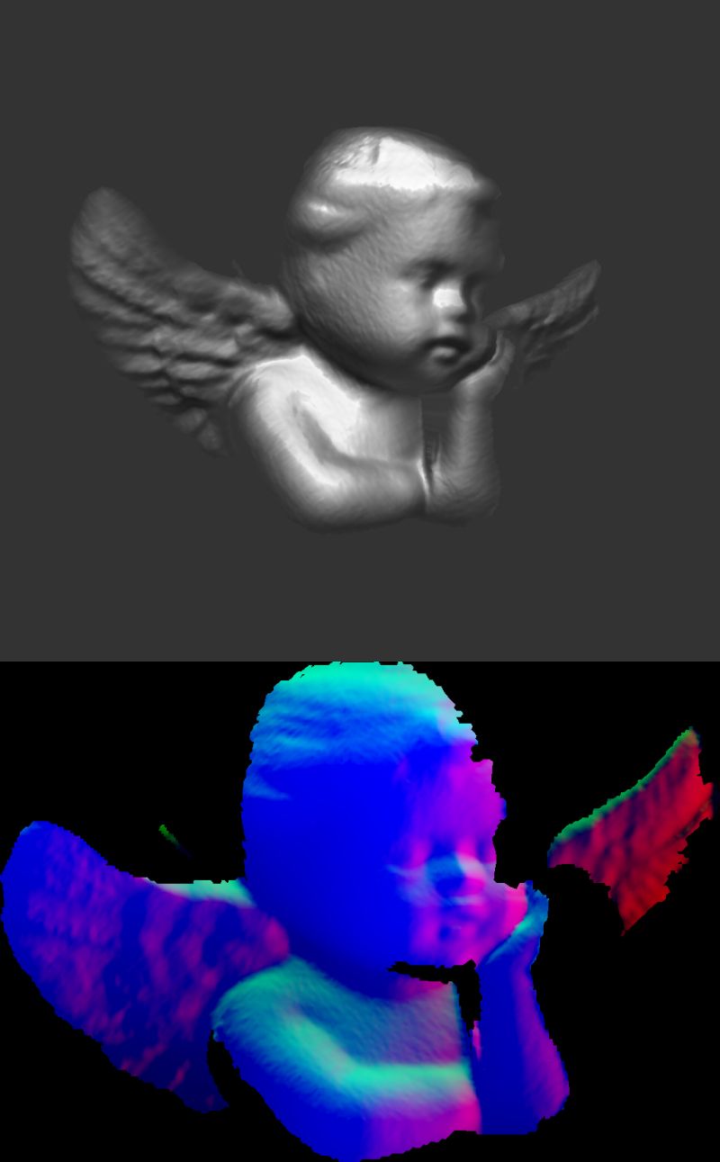
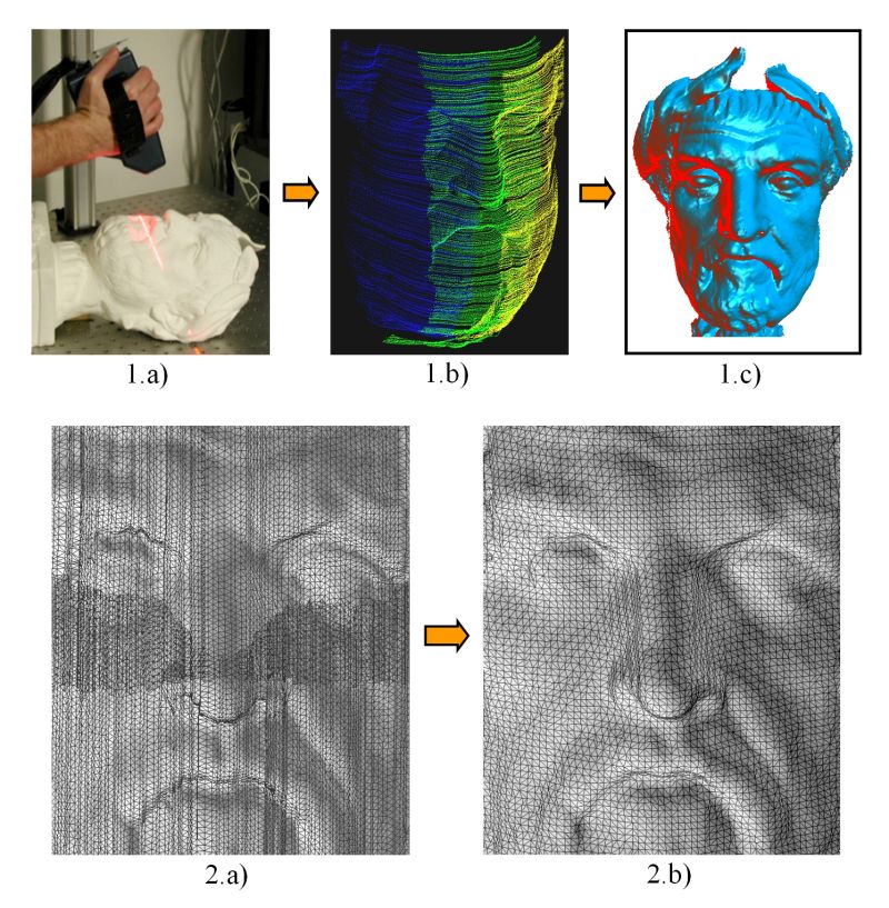
Acquisition d'objet à petite échelle par scanner manuel : Un bunny de Stanford a été imprimé en 3D (quelques cm) puis acquis par scanner manuel à lumière structurée. On voit ici le maillage géométrique et des habillages texturés.

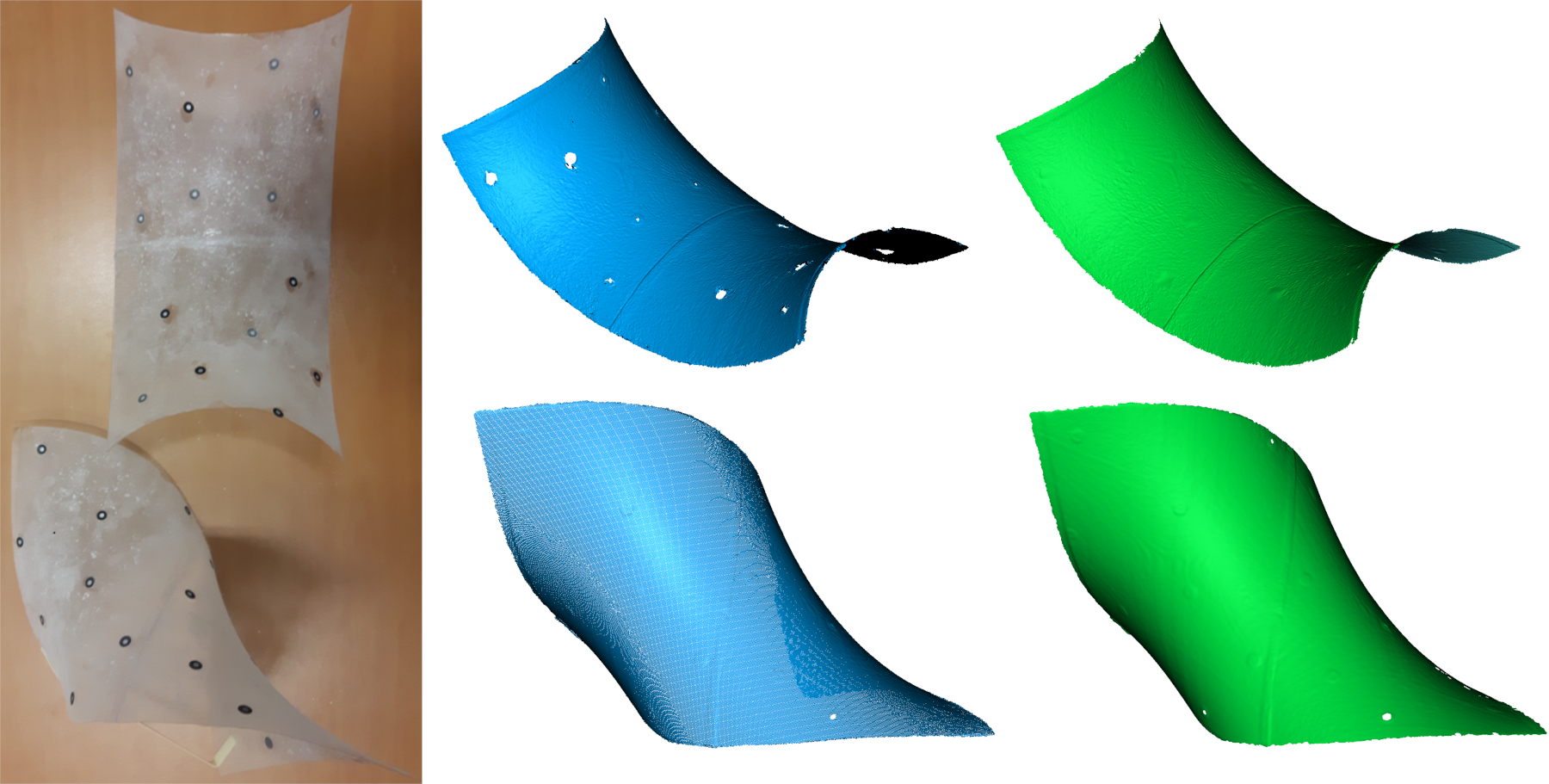
Acquisition de la géométrie fine d'objets transparents : Du talc a été déposé sur des coques minces transparentes avant de les scanner pour évaluation de modèles de déformation physique.

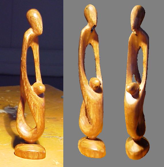
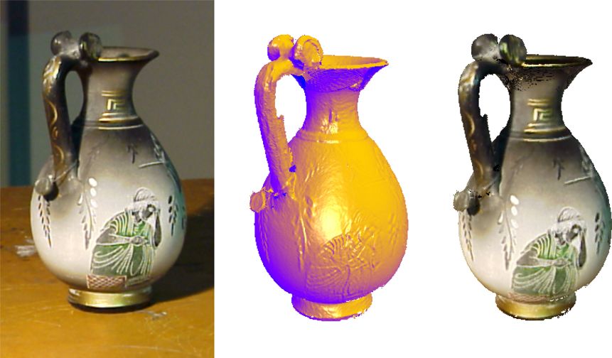
Acquisition géométrie + couleur et visualisation : Gauche : photographie de l'objet original. Milieu : la géométrie est reconstruite à partir de 5 acquisitions. Droite : rendu d'une copie synthétique.

Acquisition géométrie + couleur et visualisation : Gauche : photographie de l'objet original. Droite : deux vues synthétisées à partir de sa copie numérique.

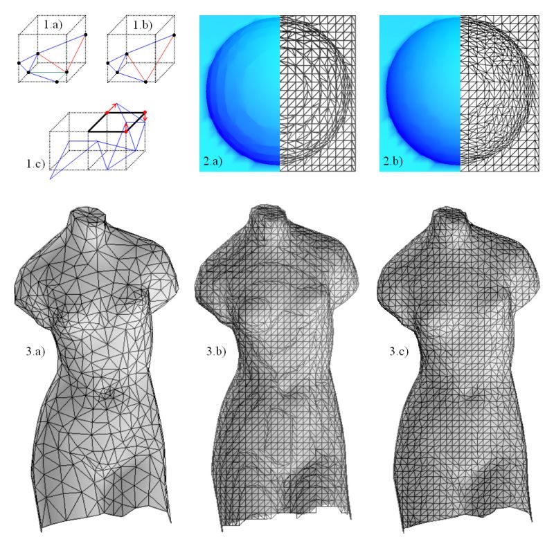
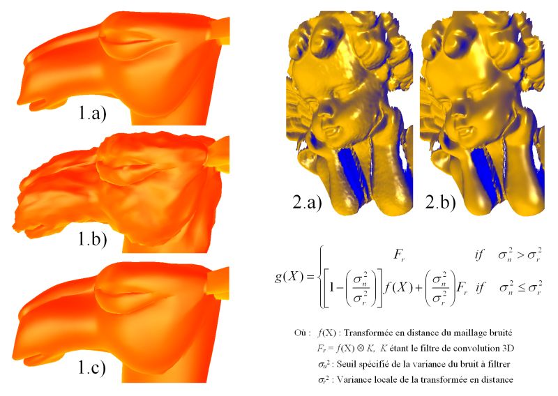
Reconstruction d'objets numérisés : Adaptation du Marching Cube et nouvelle triangulation Marching Square pour la transformée en distance vectorielle.

Reconstruction d'objets numérisés : Fusion de maillages dans le domaine de la transformée en distance vectorielle.

Reconstruction d'objets numérisés : Filtrage adaptatif de maillages dans le domaine de la transformée en distance vectorielle.

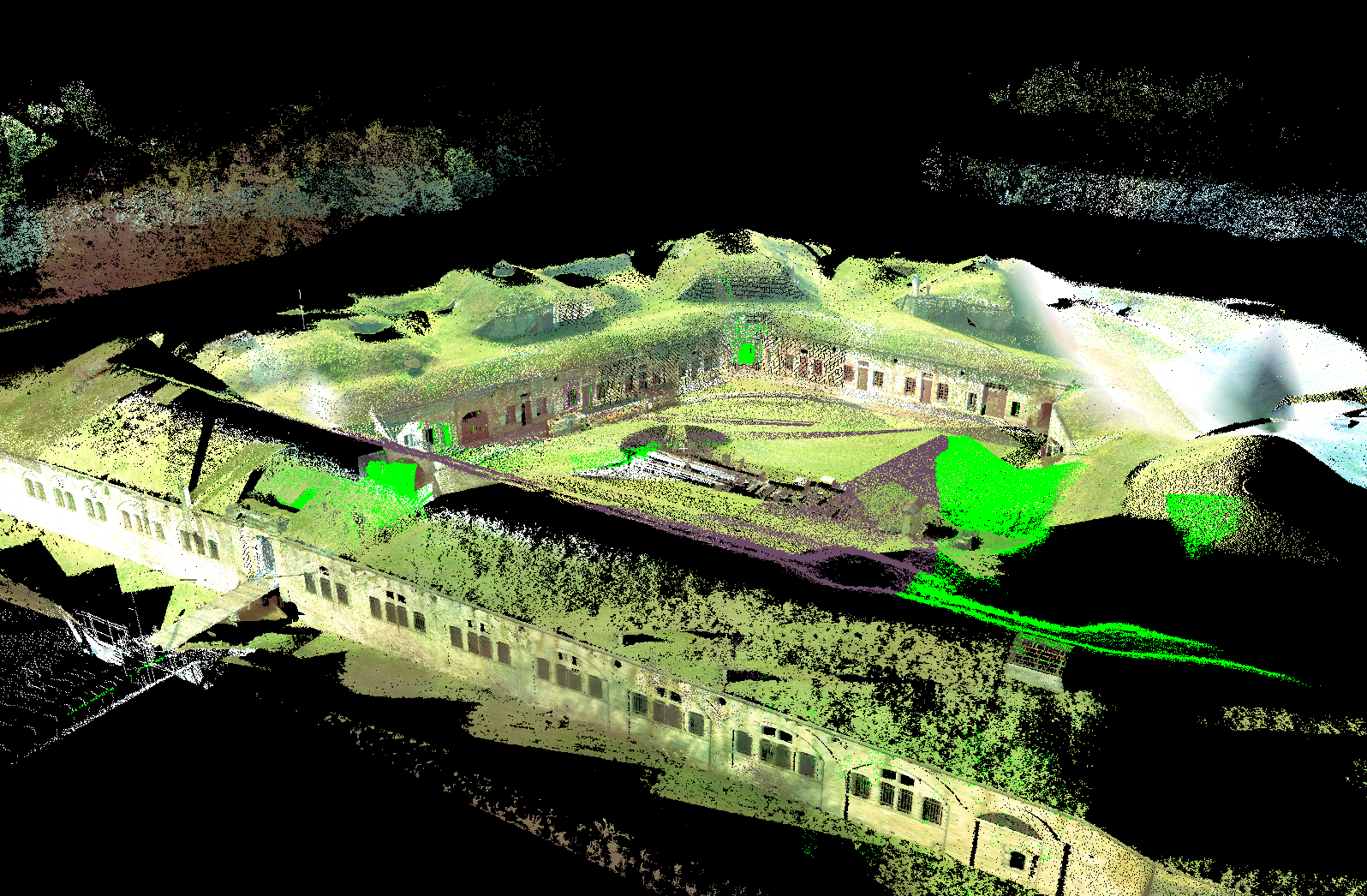
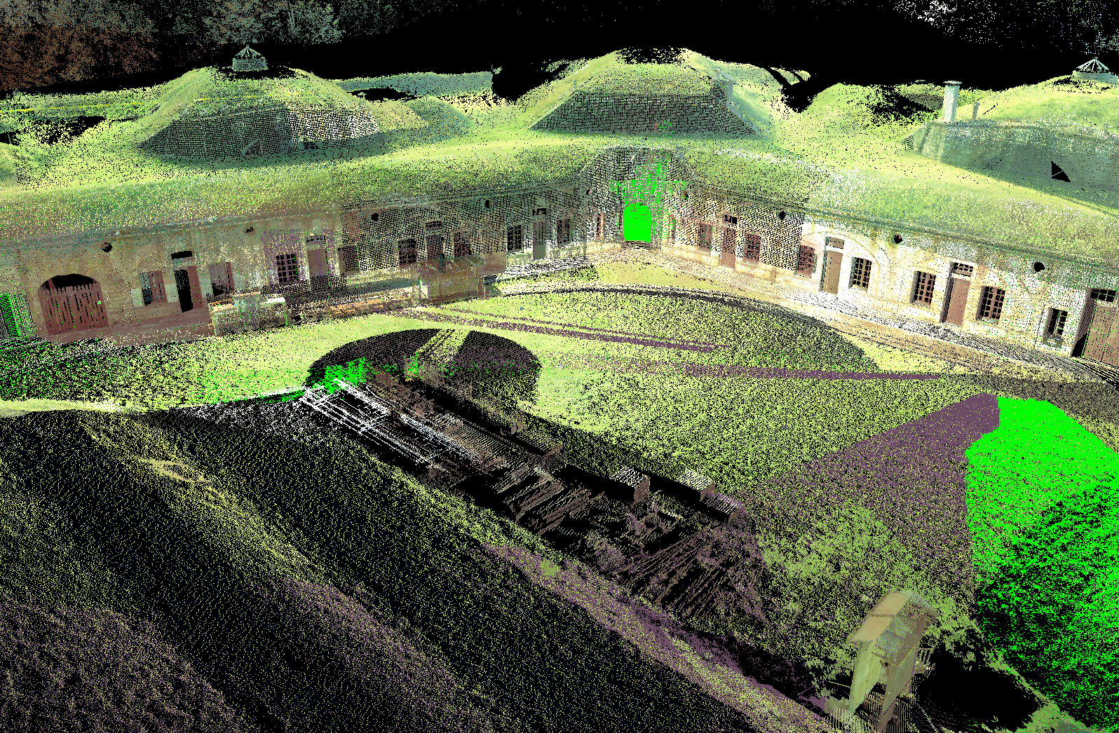
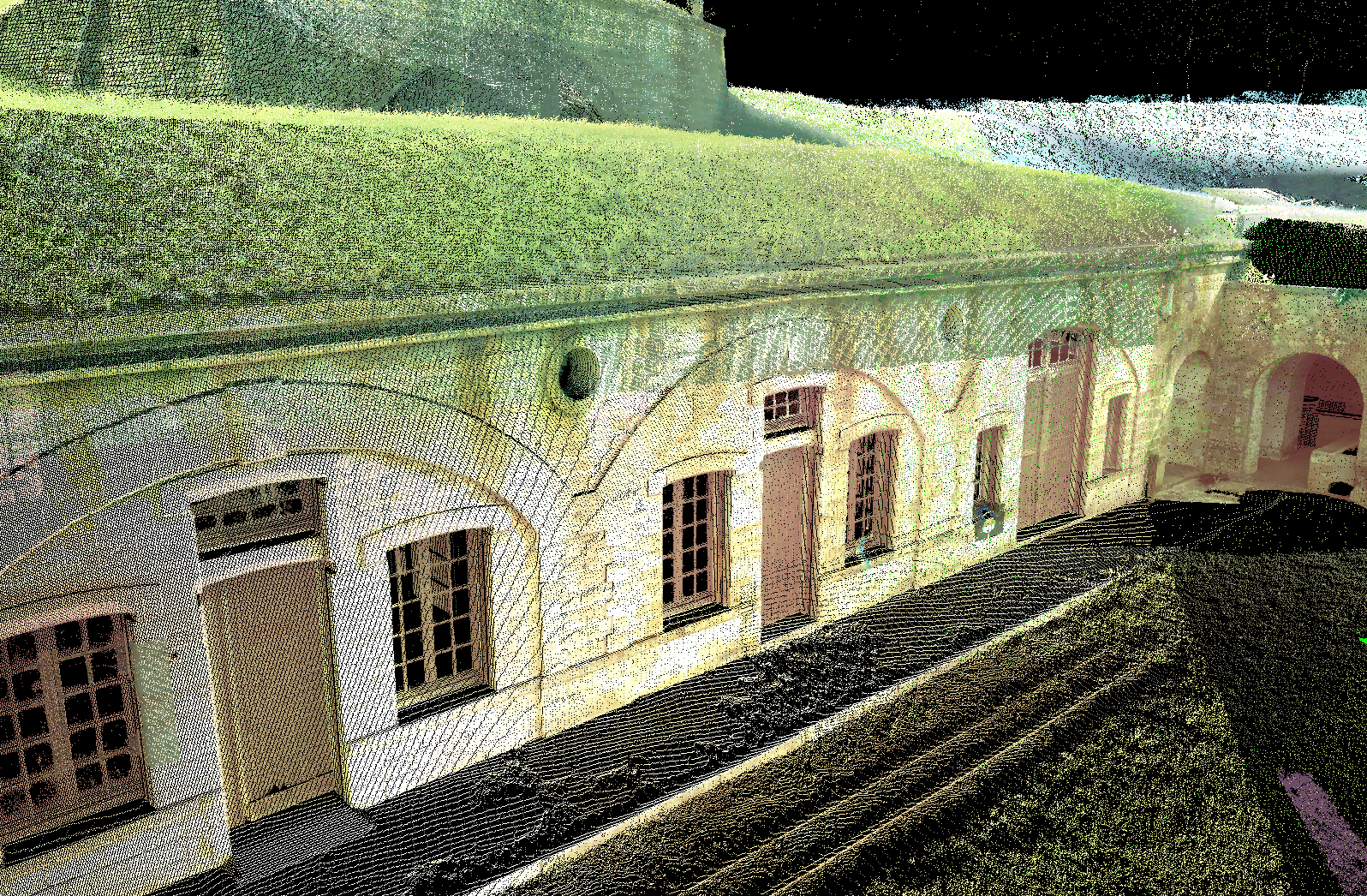
Numérisation de bâtiment : Fort Bois l'Abbé par LiDAR terrestre.

Numérisation de bâtiment : Fort Bois l'Abbé par LiDAR terrestre.

Numérisation de bâtiment : Fort Bois l'Abbé par LiDAR terrestre.

Numérisation de bâtiment : Fort Bois l'Abbé par LiDAR terrestre.

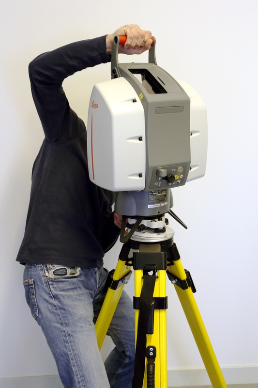
Matériel de numérisation : Scanner LiDAR terrestre.

Matériel de numérisation : Scanner LiDAR terrestre.

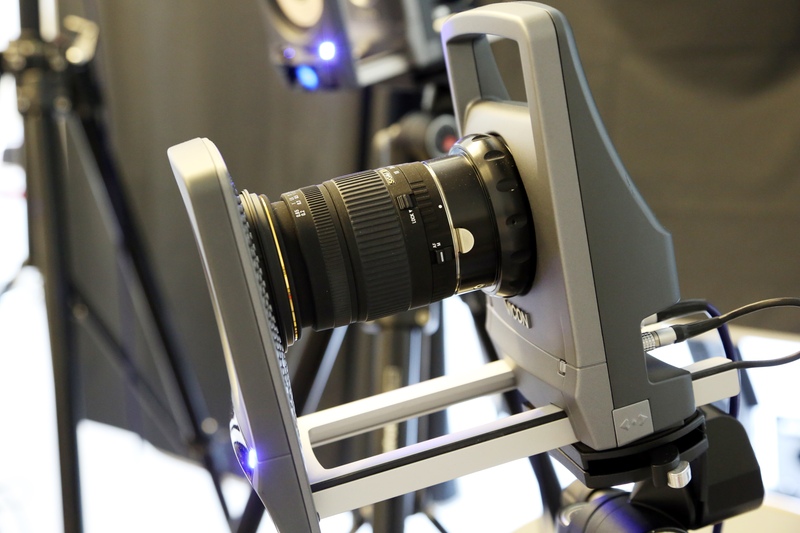
Matériel de numérisation : Capture des mouvements.

Matériel de numérisation : Capture des mouvements.

Matériel de numérisation : Capture des mouvements.


Contraintes géometriques

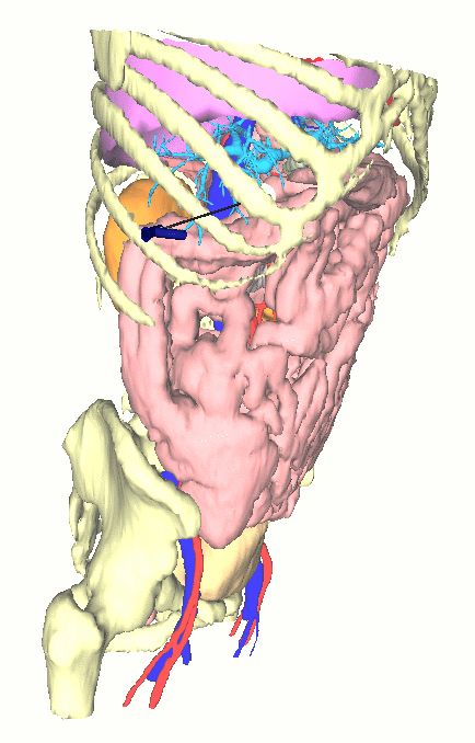
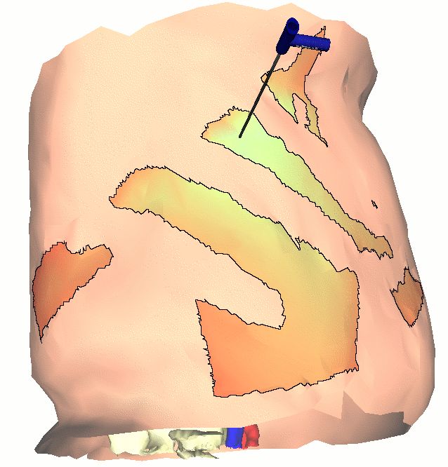
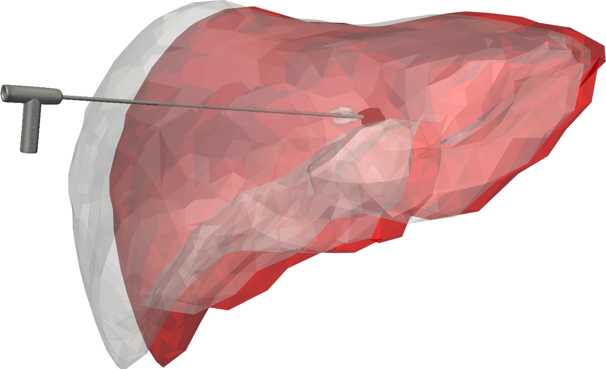
Planification d'opérations chirurgicales : Calcul automatique du placement optimal d'aiguille de radiofréquence et affichage avec transparence de la peau et du foie.

Planification d'opérations chirurgicales : Calcul de déformation de la zone de lésion de radiofréquence à proximité des vaisseaux sanguins.

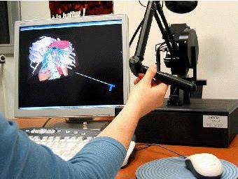
Planification d'opérations chirurgicales : Retour d'effort pour la simulation réaliste du geste chirurgical dans l'application de radiofréquence.

Planification d'opérations chirurgicales : Zone candidate pour l'insertion d'aiguille de radiofréquence avec coloration des zones selon les contraintes souples.

Planification d'opérations chirurgicales : Subdivisions des triangles à la frontière des zones candidates pour l'insertion d'aiguille de radiofréquence.

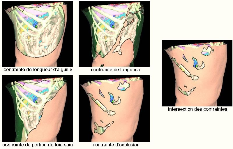
Planification d'opérations chirurgicales : Visualisation de 4 contraintes strictes sous forme de zones d'insertion - et leur intersection - dans l'application de radiofréquence.

Planification d'opérations chirurgicales : Fusion de 3 contraintes souples représentées sous forme de colorations des zones candidates pour l'insertion d'aiguille de radiofréquence.

Planification d'opérations chirurgicales : L'application de radiofréquence sur station de réalité virtuelle.

Planification d'opérations chirurgicales : Inclusion de simulations biomécaniques dans la boucle d’optimisation.

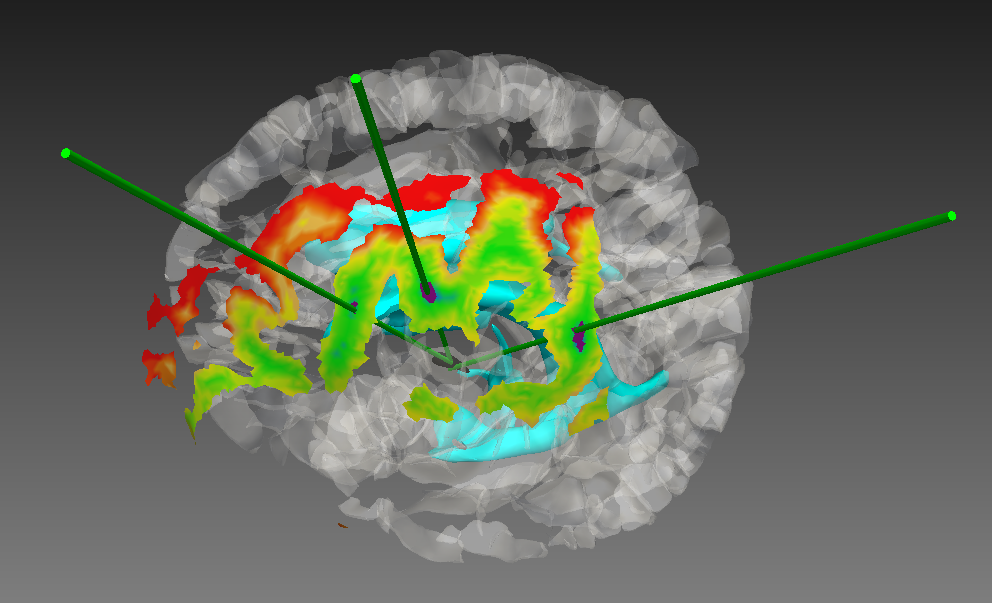
Planification d'opérations chirurgicales : Résolution de contraintes de positionnement en stimulation cérébrale profonde.

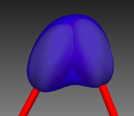
Planification d'opérations chirurgicales : Calcul de la propagation thermique en cryoablation.

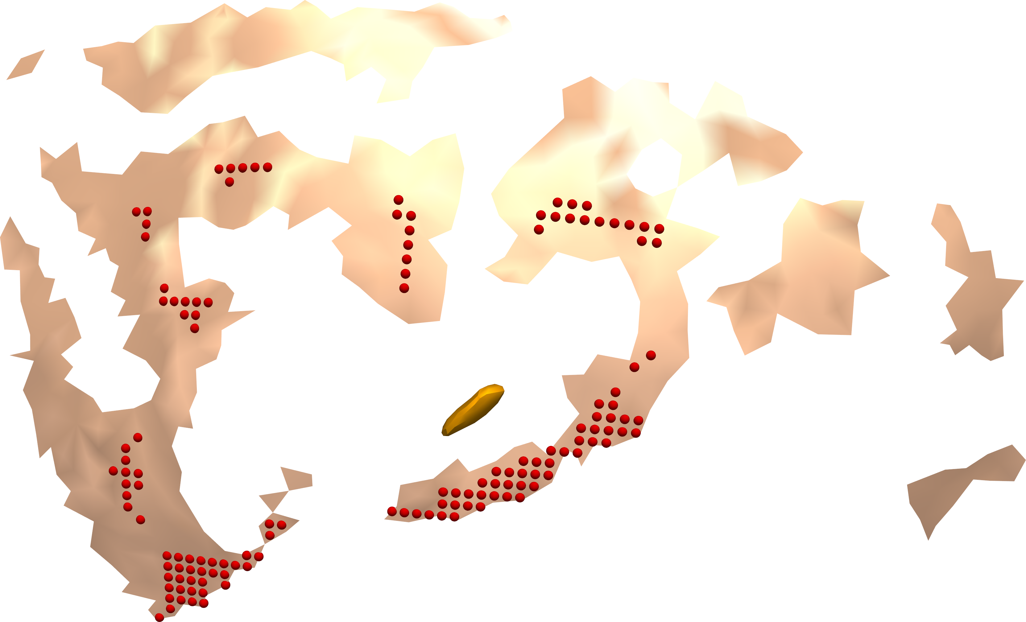
Planification d'opérations chirurgicales : Points d'insertion possibles sur un front de Pareto.

Planification d'opérations chirurgicales :

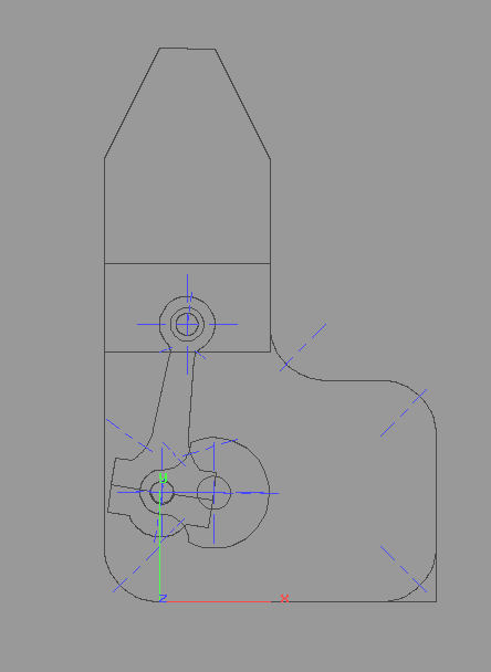
Constructions géométriques :

Constructions géométriques :

Constructions géométriques :


Intéraction

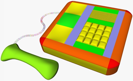
Interactions with a Hybrid Map for Navigation in Virtual Reality : (A B) interactions using the Oculus hand Controller (C D) interactions using the smartphone. The red circle represents the fingertip position in the VE. [ACM-ISS-2020]

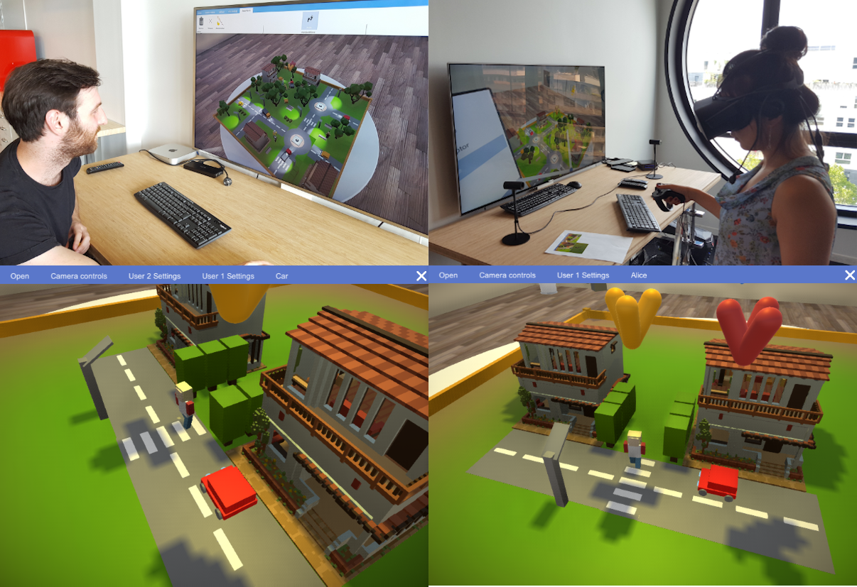
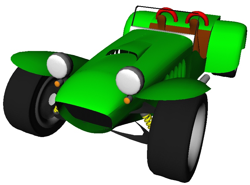
UMI3D: A Unity3D Toolbox to support CSCW Systems Properties in Generic 3D User Interfaces : UMI3D case study - social interactions. User 2 (on the left) waits for the character controlled by User 1 (on the right) to cross the road before continuing to drive the red car. [ACM-HCI-2018]

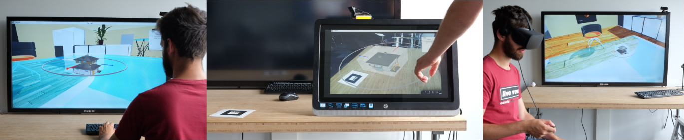
A Unified Model for Interaction in 3D Environment : A new model for designing VR AR and MR applications independently of any device. [ACM-VRST-2017]

A Hybrid Projection to Widen the Vertical Field of View with Large Screens : Left image represents a view with a perspective projection. Right image shows and example of the hybrid projection. In left image the user cannot see the chair behind him. [3DUI-2016]

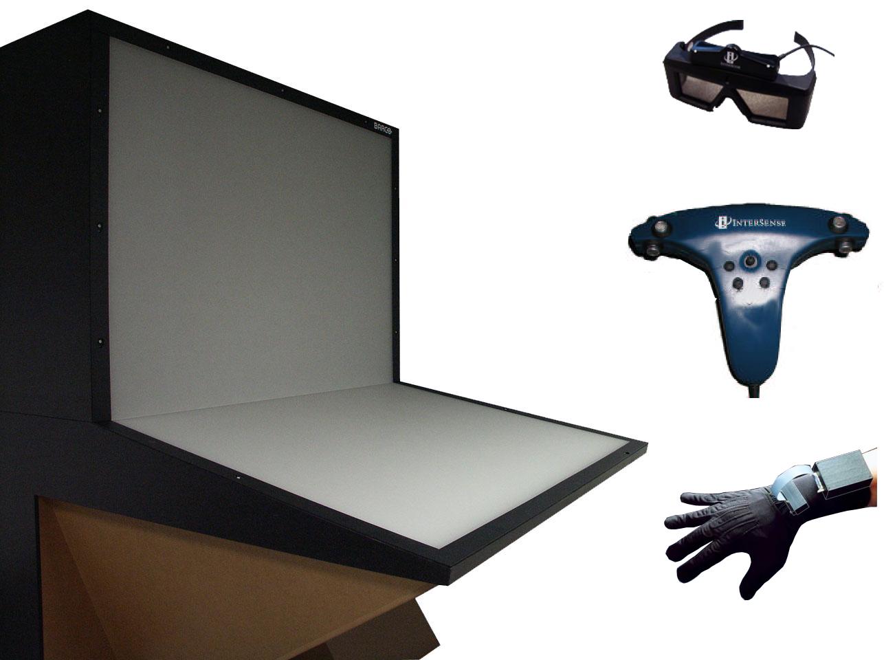
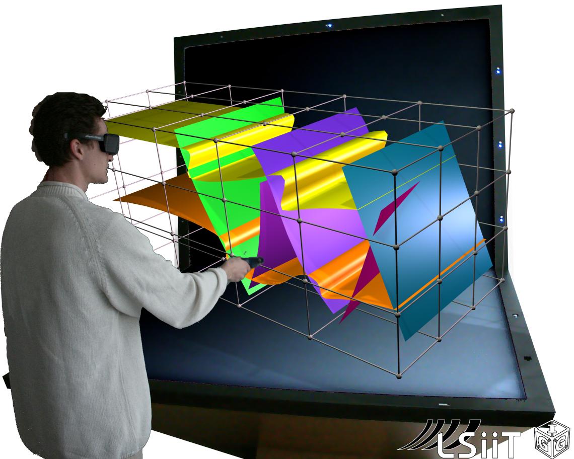
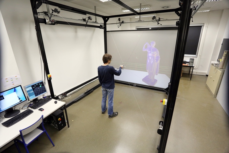
Materiel de réalité de synthèse : Spidar et workbench.

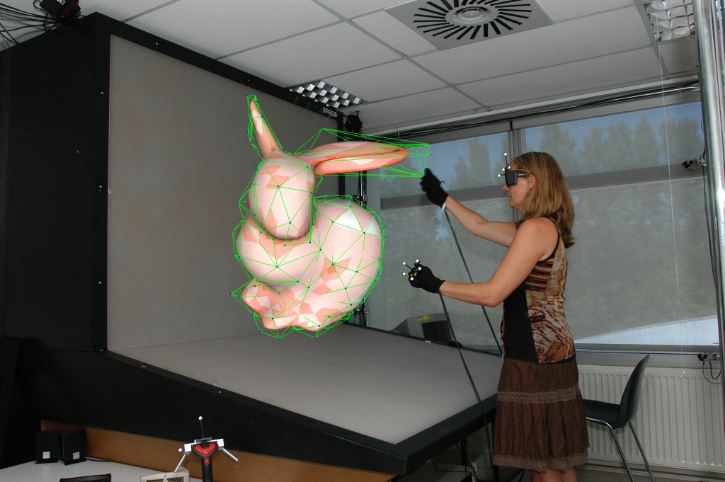
Materiel de réalité de synthèse : Gants et wand.
- Erreur lors de la création de la vignette : Fichier manquant
Materiel de réalité de synthèse : INCA

Materiel de réalité de synthèse : Effecteur du périphérique haptique

Materiel de réalité de synthèse : Caméra pour suivi de position

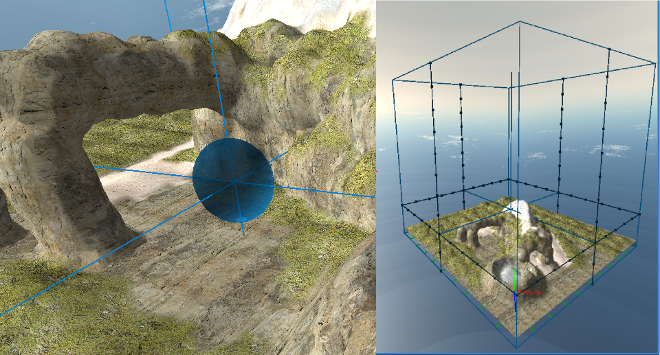
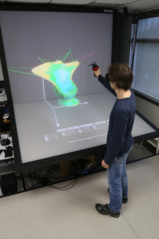
Edition de Terrain : Edition de terrain

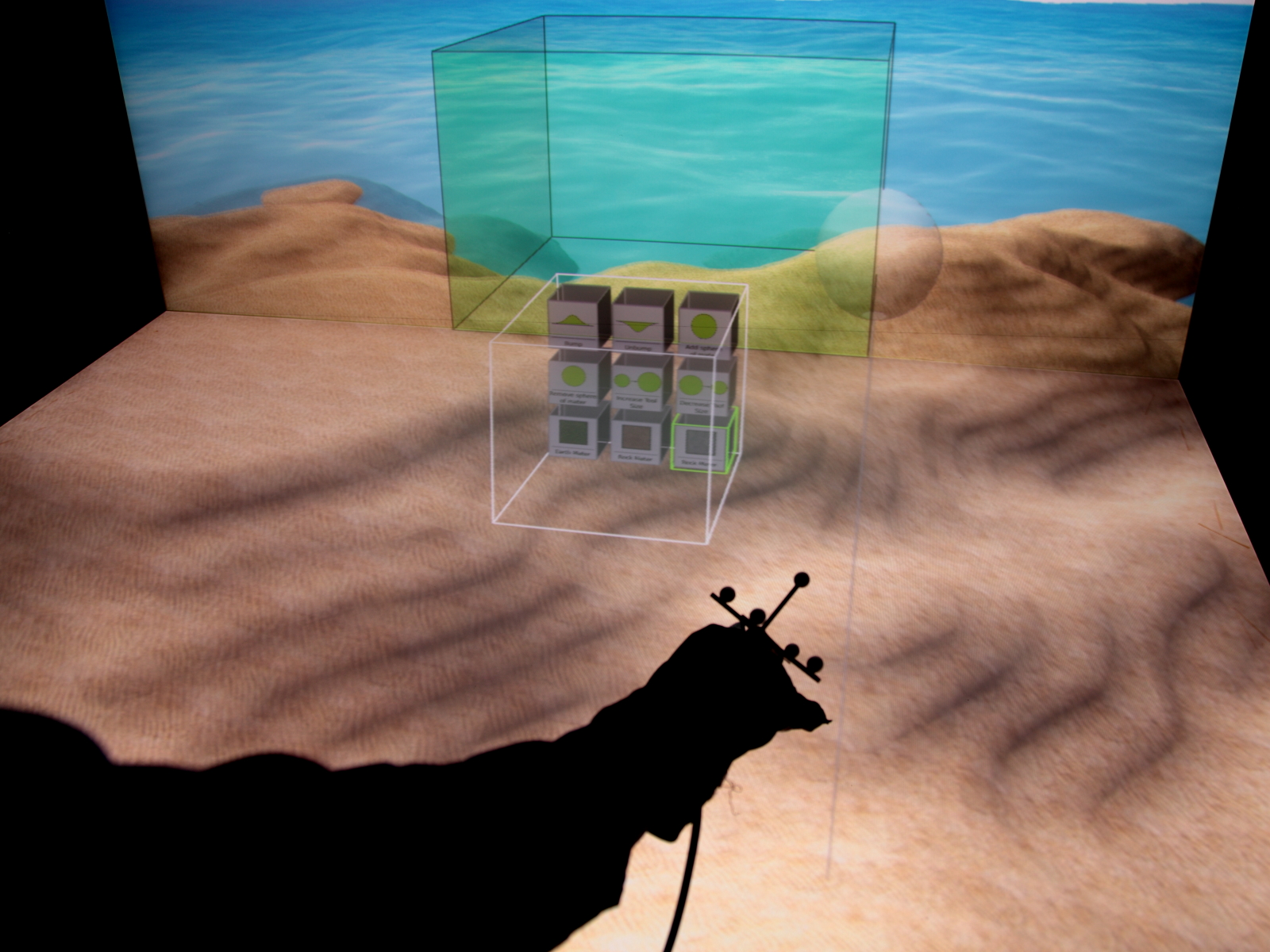
Edition de Terrain : CCube Menu

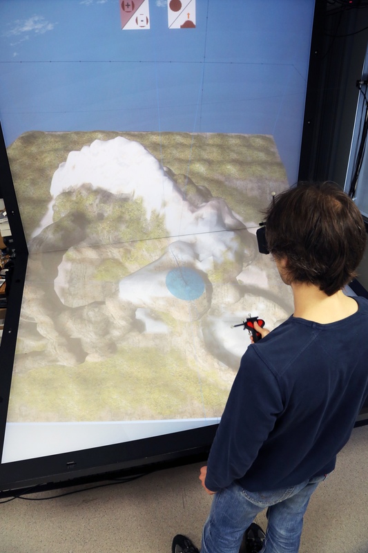
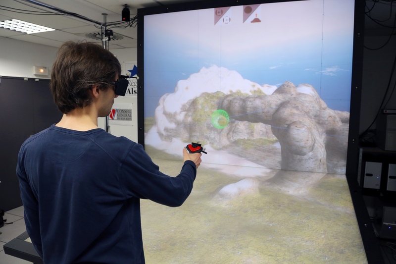
Edition de Terrain : Edition de terrain

Edition de Terrain : Edition de terrain

Applications géologiques :

Applications géologiques :

Applications géologiques :

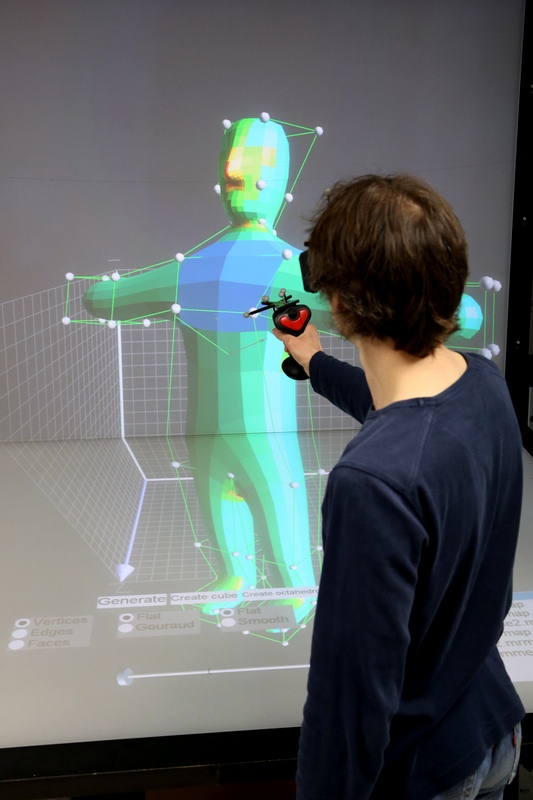
Edition multi-resolution en Réalité Virtuelle :

Edition multi-resolution en Réalité Virtuelle :

Edition multi-resolution en Réalité Virtuelle :

Edition multi-resolution en Réalité Virtuelle :

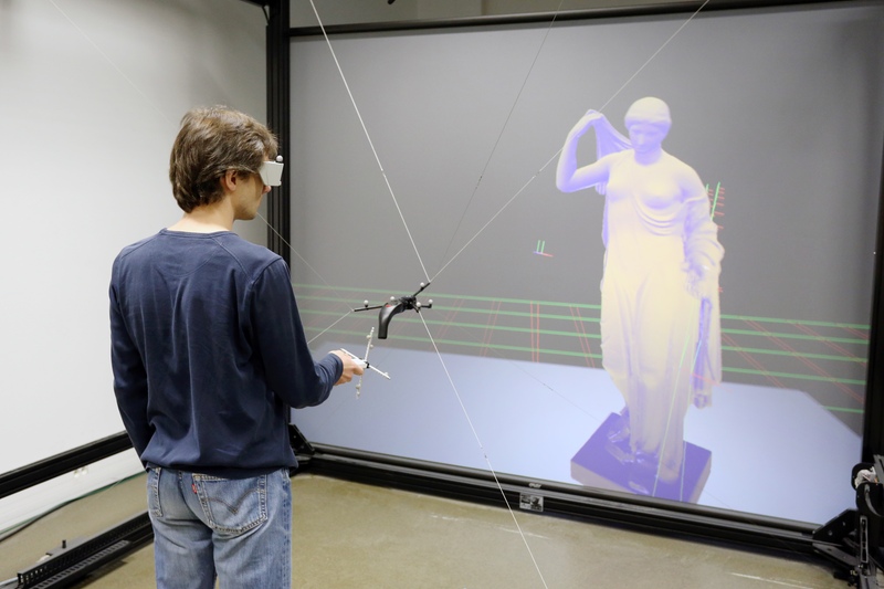
Visualisation d'objet numérisé en environnement immersif :

Visualisation d'objet numérisé en environnement immersif :

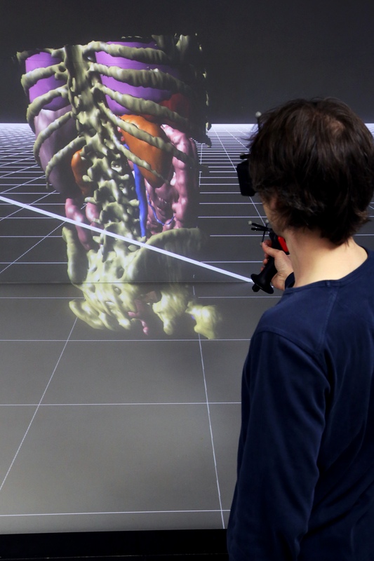
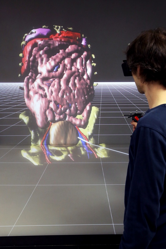
Visualisation de modèle médical en environnement immersif :

Visualisation de modèle médical en environnement immersif :

Facteurs de perception des distances en environnement virtuel : Le principe de la projection hybride et les différents paramètres utilisés pour le rendu de la scène.

Facteurs de perception des distances en environnement virtuel : Gauche : vue de scène projetée avec la projection perspective ordinaire. Droite : un exemple de la même vue avec la projection hybride. Sur l'image de gauche l'utilisateur ne voit pas les pieds de la chaise devant lui.

Facteurs de perception des distances en environnement virtuel : Exemple de visite virtuelle : des positions différentes lors de la visite d'une maison meublée. Le chemin de navigation est représenté en fil d'Ariane en vert.

Séparation des degrés de liberté pour la manipulation d'objets : Etude de l'impact de la séparation des degrés de liberté pour l'interaction en environnement immersif.


Modélisation

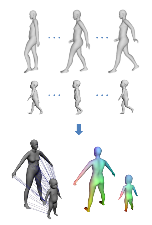
Multi-scale Space-time Registration of Growing Plants : Result of our framework on one tomato plant (left) and one maize (right): corresponding points share the same colour. Some landmarks have been sampled and are shown connected to their corresponding points. [3DV-2021]

Multi-scale Space-time Registration of Growing Plants : Point-wise matching of the whole plant growing. [3DV-2021]

Tubular shape scaffolding : Hexahedral reconstruction of the metatron mesh using the tubular shape scaffolding algorithm. [VISIGRAPP-2021]

Tubular shape scaffolding : Using the red scaffold as a support a hexahedral mesh is produced then optimized and fitted to the input surface. [VISIGRAPP-2021]
- Viville 2021 hexahedral mesh generation for tubular shapes using skeletons and connection surfaces 02.png
Hex Meshes : Construction of hexahedral meshes (yellow) from an input surface (blue) and it's curve skeleton using the scaffold method. [VISIGRAPP-2021]

Descriptive: Interactive 3D Shape Modeling from A Single Descriptive Sketch : The constraints specified by the user are shown in red for positional constraints green for corner points and green–red for both. [CAD-2020]

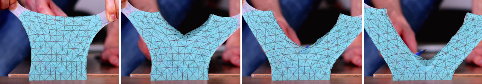
Analyzing Clothing Layer Deformation Statistics of 3D Human Motions : Comparison to ground truth. First row: our predicted clothing deformation. Second row: ground truth colored with per-vertex error. Blue: 0cm; red: 10cm. [ECCV-2018]

Reconstructing Flowers from Sketches : Reconstruction of a flower model from a sketch: input sketch (a); guide strokes provided by the user (b); segmented sketch into petals and other botanical elements (c); reconstructed model (d and e). [PG-2018]

Reconstructing Flowers from Sketches : Results obtained with our modeler. [PG-2018]

Reconstructing Flowers from Sketches : More flower model examples from our modeler. [PG-2018]

Indoor Scene reconstruction from a sparse set of 3D shots : Three shots containing no overlapping area are given as input (top row). The second row shows two different results provided by our method. [CGI-2017]

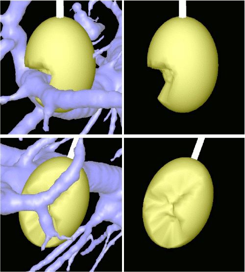
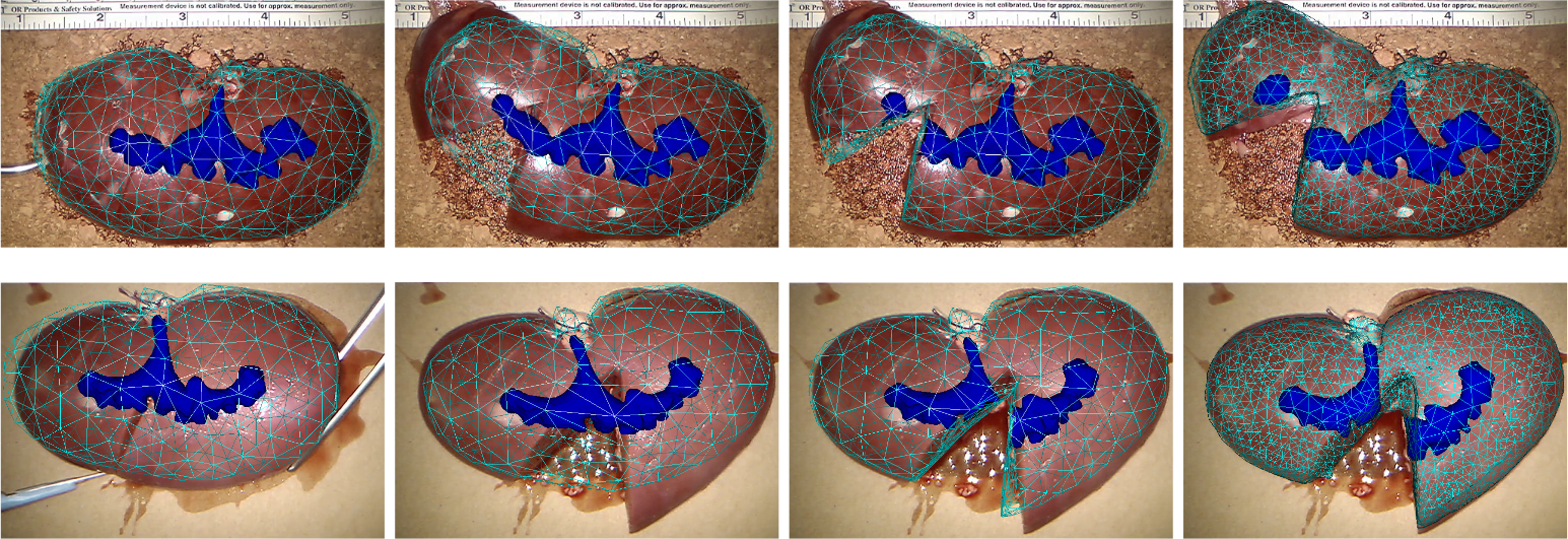
Handling Topological Changes during Elastic Registration : Augmented reality on cut and deformed kidney 1 (top) and 2 (bottom) overlaid by the virtual organ the initial registration (left) final registrations: uncut (middle left) cut (middle right) and reference registration (right). [IJCARS-2016]

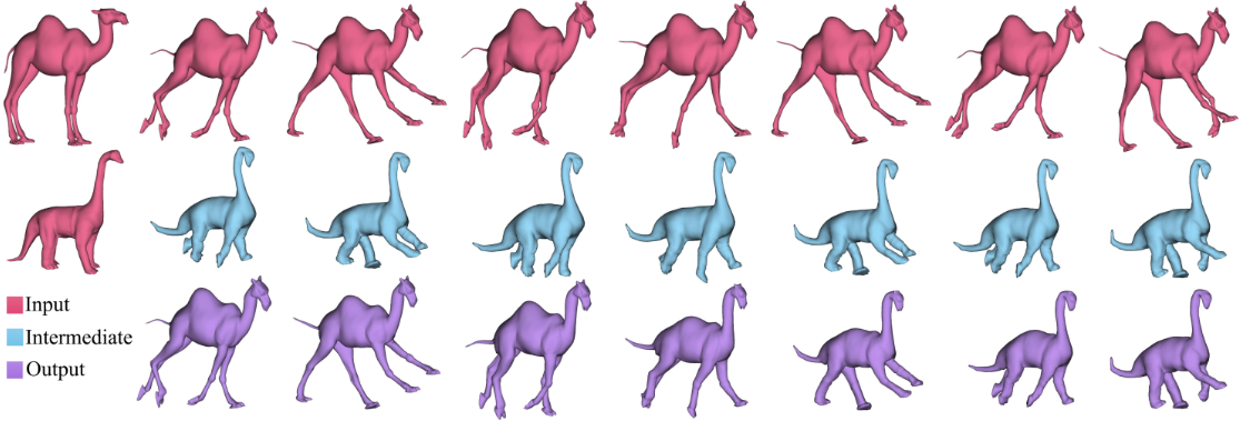
Mesh Sequence Morphing : A galloping Camel gradually changes into a galloping Dino. The Dino sequence (indicated in blue) is obtained by transferring the deformations of the Camel to the compatibly remeshed Dino in the rest pose. [CGF-2016]
- Erreur lors de la création de la vignette : Fichier avec des dimensions supérieures à 12,5 Mp
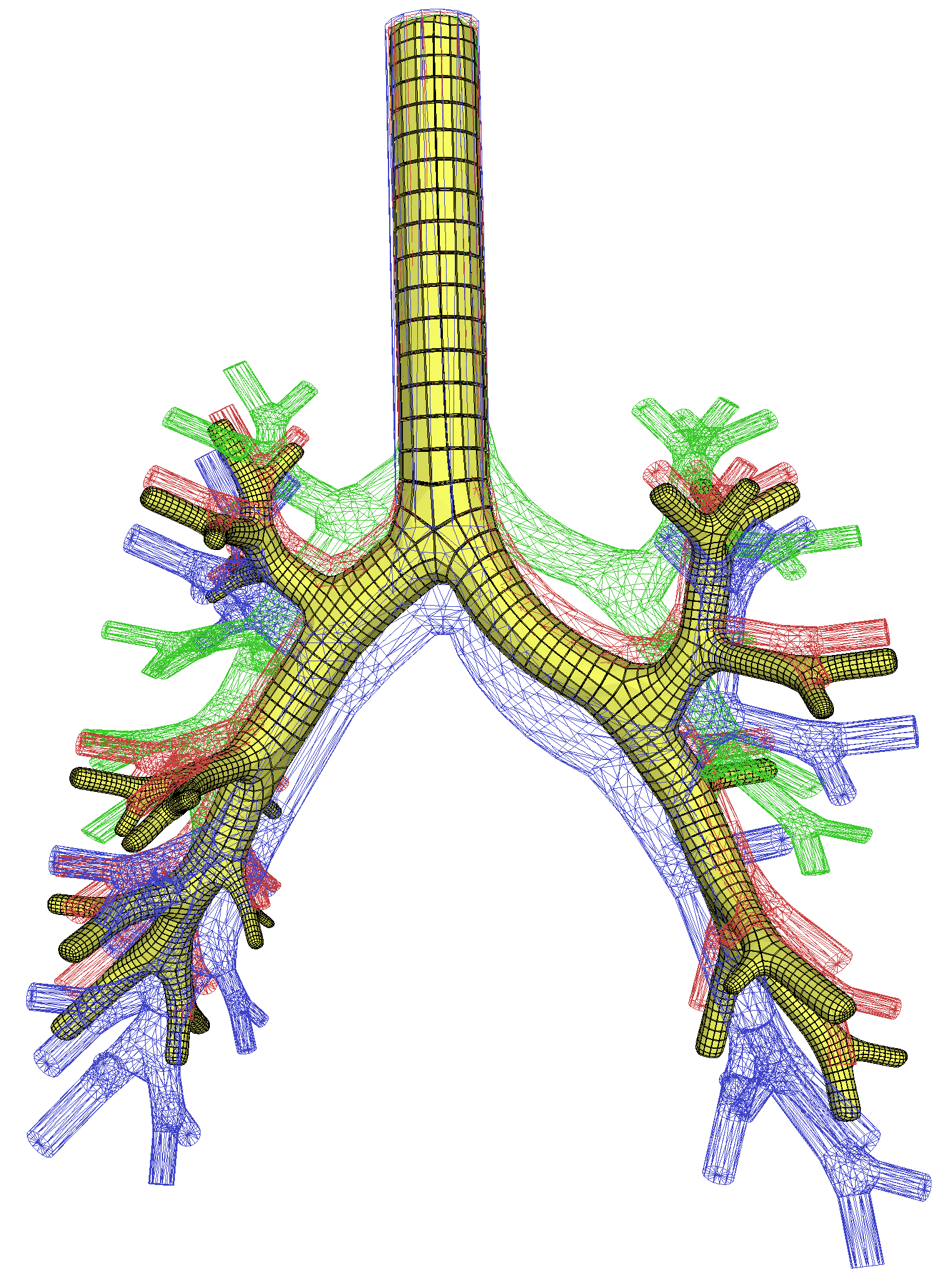
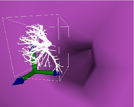
Animation de bronches : Construction d'un maillage volumique hexaédrique d'un modèle de bronches

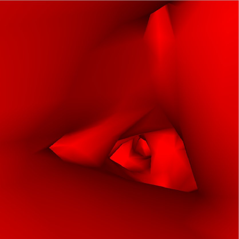
Animation de bronches : Cycle de respiration sur un maillage volumique de bronches.

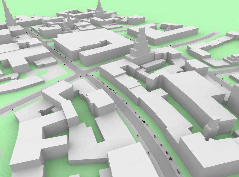
Simulation de foule : Données géographiques importées depuis open street map.

Simulation de foule : Bâtiments composés d'étages.

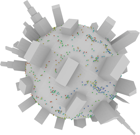
Simulation de foule : Foule sur une planète virtuelle.

Simulation de foule : Support de topologies extrêmes.

Modèle volumique adaptatif et multirésolution : Labellisation des cellules pour définir une hiérarchie implicite.

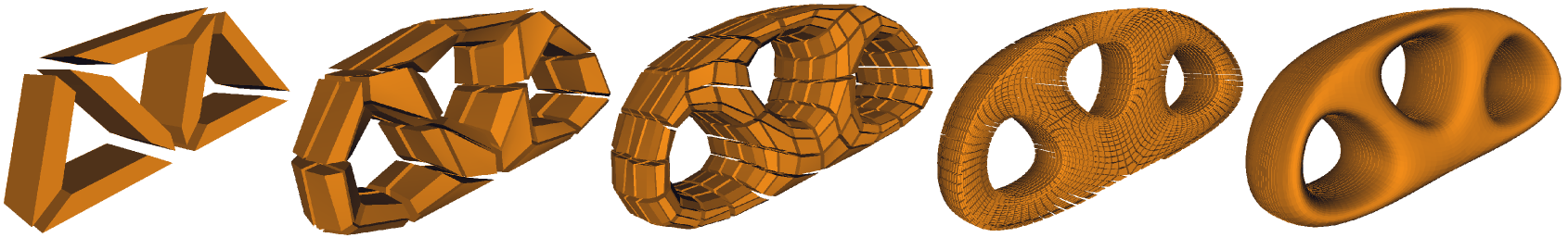
Modèle volumique adaptatif et multirésolution : Subdivision volumique d'un tore à trois trous modélisé par un ensemble de polyèdres quelconques.

Modélisation multi-résolution : Utilisation des MR-Maps dans un outil d'édition multirésolution avec des surfaces de subdivision multirésolution générées avec le schéma de Catmull-Clark (maillage carré).

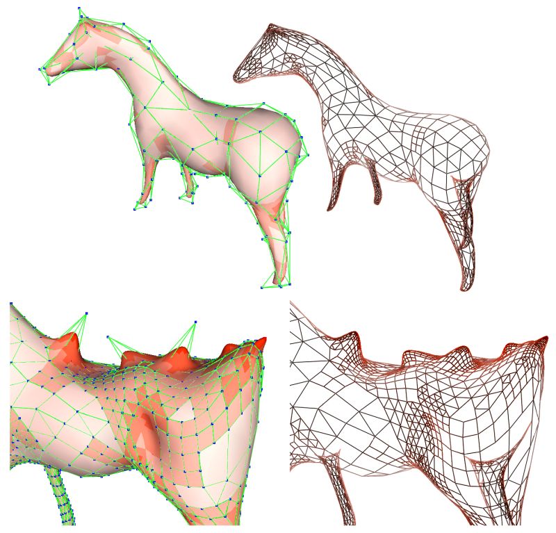
Modélisation multi-résolution : Utilisation des MR-Maps dans un outil d'édition multirésolution avec des surfaces de subdivision multirésolution générées avec le schéma Quad - Triangle (maillage hybride triangle - carré).

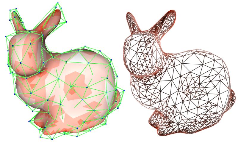
Modélisation multi-résolution : Utilisation des MR-Maps dans un outil d'édition multirésolution avec des surfaces de subdivision multirésolution générées avec le schéma Sqrt(3) (schéma de Kobbelt).

Reconstruction de maillages à partir d'images voxels : Trois étapes clés de l'algorithme de reconsctruction Delaunay Discret a) Approximation discrète des régions de Voronoï sur la frontière discrète b) Graphe de Voronoï discret c) Reconstruction par dualité : graphe de Voronoi euclidien (en noir).

Reconstruction de maillages à partir d'images voxels : Reconstruction surfacique du fameux objet dragon avec trois résolutions différentes.

Reconstruction de maillages à partir d'images voxels : Reconstruction simultanée du foie et du rein droit. La frontière commune est contenue dans les deux maillages.

Reconstruction de maillages à partir d'images voxels : Exemple de reconstruction d'un squelette et d'une aorte.

Détection et caractérisation des poches dans les protéines : Un polygone transparent met en évidence la poche principale du domaine de liaison du ligand du récepteur à la vitamine D. on peut distinguer un ligand modélisé par une union de sphères.

Détection et caractérisation des poches dans les protéines : Même protéine et même poche sans transparence cette fois. Les facettes vertes représentent un passage bloqué entre deux poches voisines. Cette information est importante pour le biologiste.

Modélisation de vaisseaux :

Modélisation de vaisseaux : Réseau vasculaire du foie reconstruit (topologiquement).

Modélisation de vaisseaux : Réseau vasculaire reconstruit (topologiquement).

Navigation dans les vaisseaux : Chemin dans un vaisseau.

Navigation dans les vaisseaux : Réseau de vaisseau.

Navigation dans les vaisseaux : Aide à la navigation.

Navigation dans les vaisseaux : Visualisation de l'intérieur des vaisseaux.

Modélisation topologie et plongement (Multifil) :

Modélisation topologie et plongement (Multifil) :

Modélisation topologie et plongement (Multifil) :

Modélisation topologie et plongement (Multifil) :

Modèles de déformation : Dogme.

Modèles de déformation : Dogme en réalité virtuelle.

Modèles de déformation : CFFD.

Simulation de découpes et déchirures en temps réel : Vue augmentée d'un objet élastique supportant de fortes déformations et des changements topologiques.

Simulation de découpes et déchirures en temps réel : Vue augmentée d'une séquence opératoire en milieu médical.

Simulation de découpes et déchirures en temps réel : Vue augmentée d'une séquence opératoire en milieu médical.

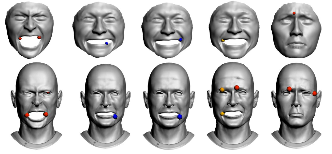
Analyse des formes - recalage - segmentation de données dynamiques : Extraction de points caractéristiques à l'aide de notre technique AniM-DoG sur différentes poses de maillages animés. La couleur représente l'échelle temporelle des points caractéristiques; le rayon indique l'échelle spatiale.

Analyse des formes - recalage - segmentation de données dynamiques : Pour un couple de maillages animés avec des mouvements similaires sémantiquement nous calculons un ensemble de points caractéristiques sur chaque maillage et leur correspondances spatiales.


Spécification et preuves

Spécifications et preuves :

Spécifications et preuves : Illustration 3D du théorème de Desargues dans un espace projectif de dimension 3 : les cotés correspondants de 2 tétraèdres en perspective l'un de l'autre se coupent en 6 points coplanaires (ces six points forment un quadrilatère complet).

Spécifications et preuves :

Spécifications et preuves :

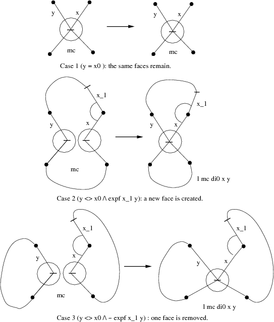
Spécifications et preuves :

Spécifications et preuves :

Spécifications et preuves :

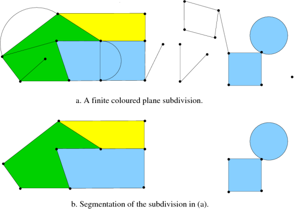
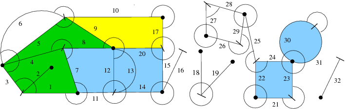
Certification d'une segmentation d'image modélisée par hypercartes colorées : Une subdivision du plan colorée (avec un sommet isolé et des arêtes pendantes) et sa segmentation.

Certification d'une segmentation d'image modélisée par hypercartes colorées : Modélisation de la subdivision précédente par une quasi-hypercarte (sommets ou arêtes ouverts).

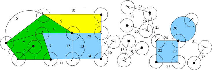
Certification d'une segmentation d'image modélisée par hypercartes colorées : Modélisation de la subdivision précédente par une hypercarte (sommets et arêtes fermés).

Certification d'une segmentation d'image modélisée par hypercartes colorées : Segmentation de la quasi-hypercarte en 2 phases (des défauts subsistent).

Certification d'une segmentation d'image modélisée par hypercartes colorées : Segmentation de l'hypercarte en 2 phases (le résultat est correct).

Illustration du théorème de Desargues :

Construction de solutions : Traduction géométrique d’une solution trouvée algébriquement.

Construction de solutions : Construction directe.


Visualisation

Importance Sampling of Glittering BSDFs based on Finite Mixture Distributions : A glittering coloured glass sphere with a spatially varying microfacet density. Left: our sampling scheme. Centre: reference. Right: Gaussian mono-lobe approximation is used for sampling. [EGSR-2021]

Edge-based procedural textures : Edges of a texture are extracted and encoded into an edge-based procedural texture (EBPT). New textures are generated either automatically or by controlling the EBPT generation by the user. [VC-2021]

Cyclostationary Gaussian noise: theory and synthesis : We convey existing stationary noises to a cyclostationary context enabling the synthesis of cyclostationary textures controlled by spectra (left) and by an exemplar (right). [EG-2021]

Procedural Physically based BRDF for Real-Time Rendering of Glints : Left: sparkling fabrics are rendered (3.0 ms/frame). Right: plane with specular microfacet density increasing. Top: our physically based BRDF (2.5 ms/frame). Bottom: not physically based [ZK16] (1.3 ms/frame). [PG-2020]

Real-Time Geometric Glint Anti-Aliasing with Normal Map Filtering : Arctic landscape with a normal mapped surface. (a) glinty BRDF of Chermain et al. [2020] prone to geometric glint aliasing. Our geometric glint anti-aliasing (GGAA) without and with normal map filtering (b and c). (d) Reference. [i3D-2020]

Semi-Procedural Textures Using Point Process Texture Basis Functions : (a) Input texture map(s) and a binary structure (b) are used to generate a semi-procedural output (d). A rendered view of the input material is shown for comparison (c). [EGSR-2020]

Modeling Rocky Scenery using Implicit Blocks : Different styles of blocks generated on a cliff and arches. From left to right tabular block style equidimensional blocks and finally rhombohedral block style. [VC-2020]

Content-aware texture deformation with dynamic control : Our deformation model allows to mimic non-uniform physical behaviors at texel resolution. Top: the parameterization is advected in a static flow field. Bottom: the deformation can be controlled dynamically. [C&G-2020]

Anisotropic Filtering for On-the-fly Patch-based Texturing : Our filtering method (right) is compared to the ground truth (middle) and no filtering (left). The ground truth is computed by an exact filtering of the high resolution. The leftmost view indicates the MIP-map levels used. [EG-2019]

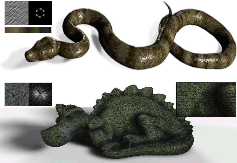
Bi-Layer textures : Our noise model decomposes an input exemplar as a structure layer and a noise layer. Large outputs are synthesized on-the-fly by synchronized synthesis of the layers. Variety can be achieved at the synthesis stage by deforming the structure layer while preserving fine scale appearance encoded in the noise layer. [EGSR-2017]

Multi-Scale Label-Map Extraction for Texture Synthesis : The input non-stationary texture (a). Hierarchy of labeled clusters: coarse scale (b) includes finer scales (c). Interactive texture editing (d) and content selection for creating new non-stationary textures (e). [SIGGRAPH-2016]

Modélisation et synthèse de textures : Des cartes de labels multi-échelles sont obtenues à l'aide de notre méthode d'analyse de textures. Une application possible est l'édition interactive de textures. [SIGGRAPH-2016]

Volumetric Spot Noise for Procedural 3D Shell Texture Synthesis : Left: uniform density. Middle: user controls density. Right: user controls orientation. In all cases control maps can be painted interactively. [CGVC-2016]

Volumetric Spot Noise for Procedural 3D Shell Texture Synthesis : Bunny1 with the "ring" kernel profile (a) and a semi regular distribution profile (b). Bunny2 with a Gaussian kernel profile (c) a random distribution profile (d) and a density map (e). Dragon and plan: use a color map (f) a density map (g) a kernel (h) and a random distribution (i). [CGVC-2016]

Procedural Texture Synthesis by Locally Controlled Spot Noise : Examples of a near-regular features reproduction by a single spot noise. Left: kernel profiles and distribution profiles. Right: blue fabric pattern applied on a 3D model. [file:///C:/Users/joris_r/AppData/Local/Temp/Pavie.pdf [WSCG-2016]]

Rendu de scintillement : A glittering copper sphere with spatially varying glitter density illuminated by an environment map and a point light. See [EGSR-2021].

Synthèse cyclostationnaire de textures :

Visualisation volumique avec éclairage :

Visualisation volumique avec éclairage :

Visualisation volumique avec éclairage : Occlusion ambiante.

Textures : Texture volumique.

Textures : MegaTexel texture.

Textures : Scène complète.

Visualisation volumique accélérée par GPU : Rendu d'objet transparent via un algorithme dérivé du relief mapping assimilable à un lancé de rayons sur un champs de hauteurs. L'objet est simplement représenté par une combinaison de cartes de hauteurs.

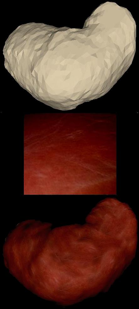
Visualisation volumique accélérée par GPU : Rendu d'un objet scanné via un algorithme de relief mapping. On s'attache ici à visualiser l'objet en exploitant directement les données issues de scanner 3D sans utiliser de. Haut : rendu obtenu. Bas : carte de hauteurs et de normales.

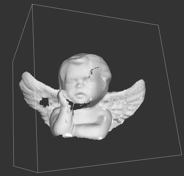
Visualisation volumique accélérée par GPU : Rendu via un algorithme de relief mapping d'un objet complet scanné : aucun maillage complexe n'est utilisé. Seul un cube sert de support au rendu.

Visualisation : Rendu d'un foie texturé.

Visualisation :

Visualisation : Rendu de matériau transparent.

Visualisation : Rendu de fluides.

Visualisation : Rendu de bijoux.

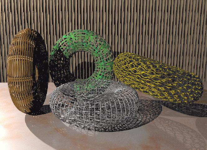
Modélisation et synthèse de textures : Des textures sont synthétisées à la volée sur GPU à partir d'échantillons d'exemples à plusieurs échelles.

Modélisation et synthèse de textures : Des textures sont synthétisées à la volée sur GPU grâce à une analyse spectrale.